
3D Sensor SPMs
3D Topography x time sensor SPMs can help you identify the latency and location of effects in sensor space. For example, here's a word-pseudoword effect (N=19) on magnetometers and gradiometers (RMS), thresholded for height (p<.001 unc) and extent (p<.05 corr):

Note that the code below applies to SPM5. The same general logic applies in SPM8, but the function names sometimes differ, and there is increased functionality (eg for finding the sensors closest to SPM x/y coordinates; see SPM8 manual demos for an example).
Creating 3D Sensor SPMs
1. Select averaged (m*.mat) data. (Note you can do a similar analysis within a single subject by writing images of epochs -- e*.mat -- rather than of the average). Compute gradiometer-magnitude (RMS; see note below) using one of:
(a). If your file contains both magnetometers and gradiometers: Split it into separate files for magnetometers, gradiometers, and gradiometer-magnitude (m*-mags.mat, m*-grds.mat, and m*-grms.mat, respectively).
clear S
S.D    = 'mae_mydata.mat';
S.grms = true;

spm_eeg_splitFIF(S);
(b). If your data have already been split into *-mags.mat and *-grds.mat: Compute RMS of gradiometers (*-grms.mat) using meg_grds2grms (in /imaging/local/meg_misc):
clear S
S.D        = 'mae_mydata-grds.mat';
S.do_write = 1;

D = meg_grds2grms(S);
2. Write image volumes.
% Select options (see help for spm_eeg_convertmat2ana3D):
clear S
S.interpolate_bad = 0;
S.n               = 32;
S.pixsize         = 3;
S.trialtypes      = [1 2]; % select trial types
S.Fname           = 'mae_mydata-mags.mat'; % mags

spm_eeg_convertmat2ana3D(S);

% Repeat for grds:
S.Fname           = 'mae_mydata-grms.mat'; % grds

spm_eeg_convertmat2ana3D(S);
3. Smooth image volumes (optional, but good idea for grms, since distribution of RMS of gradiometer values [over voxels] is not Gaussian, even if by Central Limit Theorem, the distribution of the mean over enough subjects will be).
% Select files (or pass from stage above)
P = spm_select(Inf,'image','Select image file(s)',[],pwd,'.*img');
% Smoothness in x (mm), y (mm) and z (ms)
SmoothKernel = [5 5 10];
for n=1:size(P,1);
           [pth,nam,ext] = fileparts(P(n,:));
           Pout{n}       = fullfile(pth,['s' nam ext]);
           spm_smooth(spm_vol(P(n,:)),Pout{n},SmoothKernel);
           Pin = strvcat(P(n,:),Pout{n});
           spm_imcalc_ui(Pin,Pout{n},'((i1+eps).*i2)./(i1+eps)',{[],[],'float32',0});
end
%The final imcalc step above is just to reinsert NaN's for voxels outside space-time volume into which data were smoothed
4. Then compute an ANOVA over subjects. Either use SPM's GUI, or a script like 'batch_spm_anova.m' which can be found in /imaging/local/meg_misc (or here http://imaging.mrc-cbu.cam.ac.uk/svn/meg_misc/devel/), eg:
% wd is your working directory (eg pwd)
outdir = fullfile(wd,'SensorTimeSPMs');
batch_spm_anova(Pout,outdir);
Viewing 3D Sensor SPMs
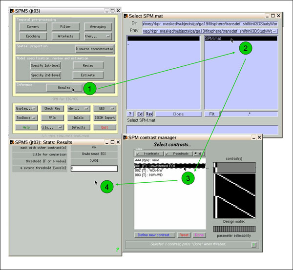
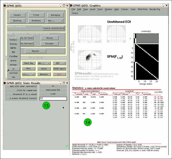
To view the results, navigate to the directory that contains the SPM.mat for your ANOVA. In an SPM window, click 'Results' (1), select SPM.mat (2), select contrast Unwhitened EOI (3), and select options: (4) don't mask, whatever title, choose your p-value and extent thresholds (I usually start with .001 and 0).
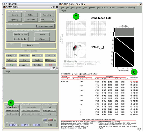
Click 'whole brain' (5) to view whole-volume results. The coordinates on the far right (6) show x (mm), y (mm), and time (ms). Ignore the glass brain images (7).
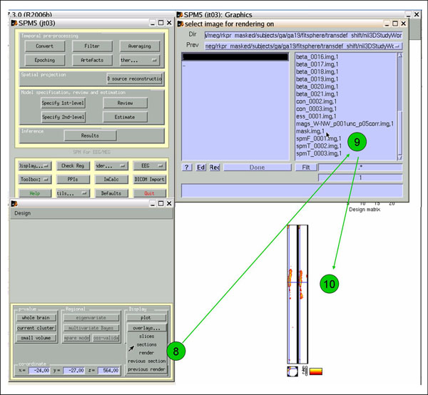
To view the cloud-in-a-box images, click 'overlays'->'sections', (8) and select mask.img (9). Lovely (10). If you want to write out the image volume, click 'save' and give it a name. You can then view it using 'Display' or 'Check Reg'.
If you want to correct for extent, rather than clicking 'Results', click 'Toolbox'->'ns'. As above, select SPM.mat, Unwhitened EOI, options: don't mask, whatever title, no p-value adjustment, threshold {p} .001 (or your choice), extent threshold 0. The leftmost column ('cluster-level p-corrected') shows p-values corrected for cluster extent (11). Note that this information was absent when you clicked 'Results'.
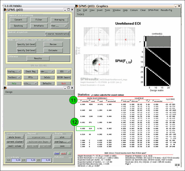
If you want to view or write out an image thresholded for cluster extent, determine what cluster size ('cluster-level k-voxel') needed to achieve your desired p-value ('cluster-level p-corrected'; in the example, 214 gets p=0.052 (12)). Then follow the above 'Toolbox'->'ns' directions, but this time enter the k-voxel extent threshold when prompted (eg., 215 (13)). Now the results are thresholded for both height and extent (14). View and save as above.
Other modalities
An F-test is often best for magnetometers (or axial gradiometers), because the polarity of the ingoing and outgoing fields is not normally of interest. Note also that the scalp location of the SPM maxima do not necessarily correspond to the locations of the underlying sources (for a dipolar pattern, the source is actually mid-way between the in- and out-going magnetic fields - ie might be many cm's distant from the SPM maxima). In other words, SPMs on magnetometer data are best for localising effects in time, and perhaps describing the general location of the in- and out-going flux, but any reporting x/y coordinates of SPM maxima should be accompanied by explanation of what these really mean. (Source analysis, which uses an explicit forward model, would address such localisation of course).
For the RMS of planar gradiometers (see section below), on the other hand, the location of the SPM maxima does correspond to the likely location of an underlying (superficial) source (so x/y coordinates can be more easily interpreted). Furthemore, one can use T-tests, because the sign of the RMS change can be interpreted (generally) in terms of more or less activity for a given contrast (eg difference of two evoked responses).
Finally, for EEG, the location and extent of an effect depends on the reference channel(s): in other words, the x/y coordinates of an SPM maximum can only be interpreted if the location of the reference channels is known (unless the input images represent a spatial derivative, eg Current Source Density). Furthermore, a large central effect may survive extent correction when using an average-mastoid reference, but be split into two non-significant clusters (of opposite polarity) when using an average reference. Thus while the location, extent and polarity (using T-tests) of an EEG SPM can be informative, for example in comparison to a previous study, such comparisons only make sense when the two studies are (re)referenced to the same reference channels. (This is one reason why using an anatomically-defined reference, such as mastoids or nose, can be preferable to the use of an average reference, which will depend on the specific EEG montage used (even though an average reference is often preferred for source localisation).)
A priori timewindows/sites of interest
Finally, if you have an a priori timewindow and/or an a priori set of sensors where you expect an effect, you can use Small Volume Correction (the SVC button). With this, you can specify a mask image saved from an orthogonal contrast in the same SPM analysis, or from a previous SPM analysis of independent data. Or perhaps more commonly, you can select a 3D "box". For example, say you had an a priori hypothesis that a condition effect would occur from 100 to 200ms poststimulus, then type [0 0 150] into the coordinates on the Input window, press SVC, select "box" and enter [140 160 100] as its dimensions (corresponding to an +/-70mm range around x, +/-80mm range around y, and +/-50ms range around 150ms). Obviously you can change the origin and x/y dimensions if you had a priori predictions about "where" over the scalp the effect might be (as well as "when" in time) - though see section above about interpreting scalp locations in EEG. If you have no a priori prediction about scalp location, then the x and y dimensions of your box can be made the limits of your input images (which can be determined by displaying one of them, or by typing a large number in the x and y boxes of the SPM input window, and seeing what SPM returns as the largest and smallest value in x and y).
Once you have defined your search volumne, the corrected (but not uncorrected) p-values in the Graphics window will now change (get smaller) owing to the reduced search volume. Hopefully some will be <.05 corrected for height or extent!
If you are interested in correcting for several timewindows (boxes), you can create a mask image in the way described below (thanks to Marina):
Use "mask.img" that you can find in your analysis directory and simply add zeros for the time periods that are not of interest:
img = spm_vol('mask.img');   %Read the volume
imgd = spm_read_vols(img);    %Get the data for the volume (should be 0s and 1s since this is a mask)
imgd(:,:, [1:149 201:299 401:end]) = 0; % Change to zero all the voxels that are outside my windows of interest, in this case the windows of interest are the samples 150:200 and 300:400 (corresponding to peristimulus times 200-300ms and 500-700ms, if the data are downsampled to 500Hz and there is a 100ms baseline period)
img.fname = 'mask_200-300_500-700ms.img' % If you want to save the mask with a different name
spm_write_vol(img, imgd)
Note that the 'ns' toolbox (see above) is not automatically invoked by SPM when small-volume correction is used. This means that you won't see significance values for clusters with SVC, and you can't correct for extent. Marina has suggested the following procedure to get your cluster information back:
Change line 146 in script spm_VOI.m and point to the toolbox, i.e. replace:
TabDat    = spm_list('List',xSPM,hReg,Num,Dis,str);
with
TabDat    = spm_list_nS('List',spm_vol('RPV.img'), xSPM, hReg, Num,Dis,str);
Once you save this script (with the same name), make sure it is in your matlab path and over the spm path (so that when you click SVC, it will use this script vs the other).
A note on Gradiometer RMS
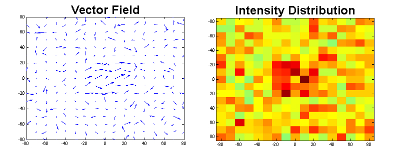
Sensor-level SPMs apply the same logic ([[http://imaging.mrc-cbu.cam.ac.uk/imaging/PrinciplesRandomFields?highlight=(field)|(random)|(theory)|random-field theory, RFT]]) as for fMRI data to MEG data, except that the image "volumes" do not consist of "voxels" in 3D-space, but rather have a 2D spatial dimension (locations of sensors) plus time as a 3rd dimension. For magnetometers, where there is one measurement per location, RFT can be applied directly. For gradiometers, however, there are two values at each location, because the gradiometer data reflect in-plane gradients (x,y) in two orthogonal directions. It is not straightforward to apply RFT (and e.g. define criteria for "smoothness") to such "vector fields". One could perform SPMs on each gradient direction separately, but this direction varies across locations with respect to the brain, so is not particularly meaningful. Furthermore, if the signal were present in both x and y directions, separate tests may be less sensitive than a combined test. It is therefore desirable to find a way of combing the two gradiometers values at each location. A common way of doing this the "Root-Mean-Square" (RMS): rms(x) = sqrt(sum(xᵢ²)/N), or for each gradiometer simply rms(g) = sqrt(sum(g₁²+g₂²)/2). This "rectification" of the signal removes information about its sign, or the direction of the gradient at each location. This is illustrated in the following images, where the left one respresents the original measurements of a gradiometer array (each arrow representing the two values of two gradiometers at one location), while the right one shows the RMS distribution computed from this vector field. The RMS values only reflect the length of the arrows, but not their orientation.
However, RMS (or any other rectification procedures) skews the distribution of original values toward positive values. Therefore, noise will not cancel when averaging the RMS (roughly speaking, positive and negative values do not cancel each other, but actually add up). To see this, consider that each measurement, y, is a mixture of signal (s) and noise (n), i.e, y=s+n (under additive noise assumptions). Let's assume, as typical, that the noise is zero-mean and Gaussian. Therefore, when averaging across many trials or subjects (observations of y), the expectation value <n>=0, and <y> approaches the true signal, s (in fact, the Signal-to-Noise ratio, SNR, increases with the square root of the number of trials). However, when you compute the signal power (part of the RMS), then the noise no longer cancels across trials: y² = (s+n)² = s² + s×n + n², and though <n>=0 (and <s×n>=0), n² is not zero. This means that even if there were no signal, the distribution of y across trials or subjects would be non-central (i.e, mean greater than zero).
This has implications for statistical comparisons between conditions. If two conditions are equal and have the same noise levels, i.e. s₁=s₂ as well as n₁=n₂, then the difference of signal power will be zero, (s₁+n₁)²-(s₂+n₂)²=0. However, if either the signal s₁<>s₂ or the noise n₁<>n₂, then the difference will be non-zero - i.e. a difference in noise levels can show up as a statistically significant difference between conditions! This could be the case, for example, if two conditions contain different numbers of trials. A special case is the comparison of one condition against zero. In this case, any non-zero n will introduce a positive bias, and thus increase the likelihood of false positives.
One way to minimise this problem is baseline correction AFTER computing signal power. This can get rid at least of the n² part of the individual conditions, and assuming that <s×n>~0, we should be safe. But there's a catch: This procedure assumes that the n² estimated from the baseline is a good approximation for the n² in your signal. But this doesn't have to be the case (imagine slow drifts across the whole epoch, or stimulus-induced muscle artefacts etc.). It is therefore essential that appropriate noise-reduction and artefact-rejection procedures have been applied. If you want to apply signal power and baseline correction to your MEG data, a possible script is here.
Even if you think the assumption that n₁=n₂ is valid, it is also important to remember that the distribution of RMS across any observations will be positively-skewed (non-Gaussian). In theory, this would invalidate parametric statistical tests (though some are quite robust, and the skewness depends on the ratio of fixed signal to random noise). So you might want to apply a further transform, e.g. the log-tranform.
One situation when this becomes more complex is when your stats are over subjects, but each subject has multiple trials. Normally one would take the RMS of the average across trials (for each subject), since the averaging will reduce the amount of noise (i.e, increase the SNR, as explained above). Therefore the distribution across subjects of this RMS value will be non-Gaussian (skewed), and a transform may be worthwhile. However, one could also calculate the RMS of each trial, and then average those within each subject. In this case, the noise will not cancel (SNR will be worse). On the positive side however, the distribution of the *mean* of any distribution, with enough observations, will approach a Gaussian (by the Central Limit Theorem). Therefore if your statistical tests are over enough subjects, then parametric tests on the mean-across-trials of the RMS will be valid. Moreover, there will be no bias of the mean RMS for each condition by the number of trials in that condition (i.e, useful for unbalanced designs). In the SPM demo script here SpmDemo, both possibilities of 1) averging across trials then taking the RMS for each subject, and 2) taking the RMS of each trial and then averaging for each subject are illustrated (the latter is just commented out).
For further information about the gradiometer RMS issue, see SensorStats.
