Slice display
This is a very brief description of my matlab slice display routines.
Please note that the most recent version of this software is incorporated into SPM5, as the slover (slice overlay) object. For older versions of SPM, please download and install the routines here.
The routines here are installed at the CBU; for those outside the CBU, the slice_overlay.tar.gz archive is available for download. Unpack the archive into a directory on your matlab path; see the archive extraction page for detailed instructions. The routines use SPM functions, so you will need SPM on your matlab path also; see the SPM home page for instructions on downloading and installing SPM.
What it does
The slice_overlay program - or equivalently the slover program in SPM5, shows images in a series of slices in a matlab figure window. It can be used to display a single image, such as a structural scan, or a composite image, where activation has been overlaid on the structural scan. Below is an example of the sort of output it produces.
This image is an example of a transparent colour overlay; however, it can produce split colour overlays of the sort often used in functional imaging:
and can combine different activation maps on the same image - for example positive and negative activations:
How to use it
Here are step by step guides to getting the effects of the type shown above. In order to follow the examples, you might want to download the slice overlay example images, and extract the archive into a directory somewhere. For all the following examples, it is easiest if you first start up matlab with SPM on your matlab path, and start SPM, so that the three SPM windows are showing, including the large "Graphics" window on the right.
Single scan display
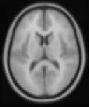
This will give you a simple slice by slice display of a given image in grayscale. The individual slices will look a bit like this:

To show slices from the single scan in grayscale, type the following at the matlab prompt:
slover('basic_ui') (for SPM5)
display_slices (for SPM2, SPM99, using the download on this page)
You will be asked to select "Image(s) to display". Select only the structural scan. If you are using the example images, select the "avg152T1.img" included with the slice overlay example images. Next the routine asks you what type of image this is. Select "Structural" from the menu. Select your image orientation (Axial/Coronal/Sagittal) - say Axial.
Specifying slices
At this point you need to type in the slices (in mm) you want displayed. By default the program suggests all the slices in the image. You can enter many slices automatically using the matlab colon notation; for example, if you wanted all slices at 6mm intervals between and including -12mm and 72mm, then you could type in "-12:6:72". To see only slices at 34 36 and 38 mm, you could enter "34 36 38", or "34:2:38". Slices can be in any order, and at any separation; for example "-10 -15 40 30 70" would show you those slices arranged in that order. When you press return, the routine displays the image slices in the SPM graphics window.
True colour activation overlay
This corresponds to the first figure on this page - a continuous wash of colour representing a range of activation values from negative to positive, shown as transparent colour on top of a gray scale structural image. This is an example slice of this type of image:

To achieve this effect, run slover('basic_ui') (SPM5) or display_slices (SPM2) again from the matlab window. Choose two images this time, the structural image - say "avg152T1.img" from the example images, and some image with continuous activation values from negative to positive. The contrast image "con_0100.img" in the examples is one such. Choose "Structural" as the type for the structural image, and "Truecolour" as the type for the activation image. For the truecolour image, the routine asks for a colormap to use. The default "actc" colormap is a reasonable choice here.
Specifying colormaps
The colormap can be the name of a matrix in the workspace, a function returning a colormap, such as the matlab colormaps "bone", "hot" and "winter", or the name of a .mat file containing a colormap (although you do not need to specify the .mat extension). You can also enter "red", "green", or "blue" to get pure red / green / blue colormaps, or you can enter the colour values directly; e.g " [0 0 0; 0.2 0 0; 0.4 0 0; 0.6 0 0; 0.8 0 0; 1 0 0] " gives a very basic pure red colormap.
Image ranges
Next you are asked for the image value range relating the values in the activation image to the colormap. The first value in this box specifies the image value associated with the first value in the colormap (for example very dark blue in the colormap "actc"); the second value is the image value associated with the last value in the colormap (e.g red in "actc"). By default these are the maximum and minimum values in the image - for the example con_0010.img these values are -4.8076 and 7.5358. To make the colors symmetrical around 0 (so half the colormap is for values greater than 0, and half for less than 0), set the range to be -7.5358 7.5358.
Colour intensities
Next choose the intensity for the structural image - this is the relative intensity of the gray scale for the activation image compared to the colours of the activation image - which can vary between 0 and 1. A value of 0.6 looks good here. For the truecolour image accept the default intensity - which will be 0.4 if you entered 0.6 above.
Choose the image orientation next, which can be axial, coronal or sagittal - choose axial. As before for the structural image only, choose your slices, say "-12:6:72" for the example images.
The resulting image has a colourbar for the activation image:

This shows the relation of colour to the image intensity values.
Split colour overlay for a single activation image
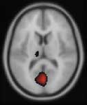
This reproduces the effect for SPM activation overlays, where the activation blobs replace the gray scale of the structural image - see the second figure on this page, and the image below:

To get this effect, choose the structural and activation images as above. Choose 'Blobs' as the image type for the activation image, and "hot" as the colormap. For the image range, set the first value to be a lower threshold for positive activation in the con_0010.img, such as 3, so the range is 3,7.5358. Choose the split colormap type, and follow the steps as above to get an image like the second figure here.
Split colours from more than one activation (deactivation) image
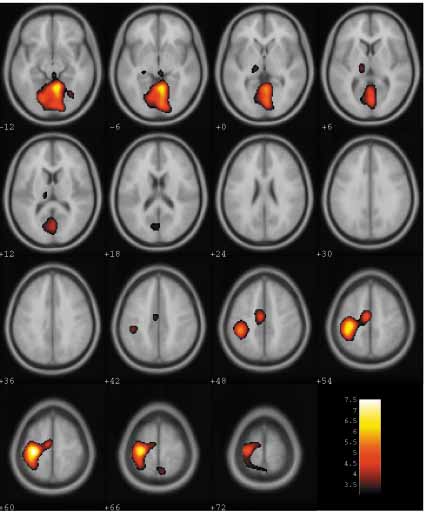
You can also show activations from more than one experiment or contrast, or activations and deactivations - shown in the third figure on this page and the example slice below.

Run slover('basic_ui') or display_slices as before, select the structural image, then select more than one activation image. Here we might wish to show activation and deactivation, so we select the activation image - say con_0010.img, then, before clicking Done, move up a directory, back to the directory containing the activation image, and select it again, so you have selected the same image twice. Choose Done now. For the first activation image, proceed as above: set the image type as "Blobs", with the "hot" colormap, and range as before. For image 2, set the type as "Negative blobs", use the "winter" colormap, and set the range to be for negative values, such as -2.5 -4.8076.
Using display slices with the SPM results section
This is the situation where you have used the SPM results interface to generate an SPM filtered map, including the glass brain views, and you want to use display_slices to overlay the results on a structural scan. You have two options. This first is to write out any thresholded etc results from the SPM results interface using the "Write filtered" button in the SPM lower left window. Thence you can use the resulting images to display as above. Alternatively you can run slover / display_slices after getting the results up in the SPM main window, select the structural scan only, and then choose the "Structural with SPM blobs" option as the image type. This finds the SPM results matrices in the matlab workspace, and displays them as a blob map (as above) using the "hot" colormap.
Simple single image or 3D matrix display
In the archive there is also a stripped down version of the display_slices routine, that merely displays all axial slices of a single image in grayscale. You can call it by typing show_image in the matlab window, and selecting an image, or with show_image('my_image.img') to display a named image file, or show_image(A) to display a three dimensional matrix "A" as an image.
A word to the wise
For those who can do matlab, there is a great deal of customization you can do with these routines - for example, show slices at arbitrary angles, return coordinates in mm of clicked points on the images, return intensity values from all the images at a certain point, and so on. For example, the slice displays can be easily batched.
Configuration for `slover` (SPM5) displays
You can then manipulate the 'so' object directly, and redisplay - e.g.
so = slover('basic_ui')followed by
so.slices = [-2:10:52];
so = paint(so);
to change and redisplay. See:
http://marsbar.sourceforge.net/doc-spm/spm5/spm5/@slover/index.html
and
http://marsbar.sourceforge.net/doc-spm/spm5/spm5/@slover/slover.html
for some documentation on the slover routines.
Configuration for `display_slices` (SPM2 / SPM99) displays
This is very similar to the slover routines. The example above becomes:
display_slices
followed by
global SO
SO.slices = [-2:10:52];
slice_overlay;
to change and redisplay. See the SliceOverlayHelp for more documentation.
There is also a script called "split2_display.m" in the archive as an example.
Printing or saving your display
If you want to print the slice overlay figure window, do so with the SPM print button, or a call to the slice overlay print function
slover('print')
slice_overlay('print') (SPM2)
The SPM and slice overlay print routines fix some odd problems with matlab postscript files.
Using spm_orthviews for true colour overlays
You can also use the latest version of the SPM display utility for showing an axial, coronal and sagittal section which you can navigate with the GUI. The routine is spm_orthviews.m, written by John Ashburner. The routines has an undocumented feature that allows you to overlay a transparent (truecolour) image over a structural. Here is an example of what this looks like:

To use this version of the routine, you replace the current SPM version of the routine with this file, start SPM 99, display a structural image with the Display button, and then add an activation overlay with the following at the matlab prompt: spm_orthviews('addtruecolourimage') after which you follow the prompts to select the activation image, and the colormap, as for the truecolour image example above. The standard SPM results GUI with the overlay button, sections options achieves the same sort of functionality using the split colormap effect.
End of examples
That's it for examples, however, a little bit of experiment may show you that the program can be persuaded to show you a very wide variety of different overlays. I hope the program is useful; please let me know of any bugs or inconveniences.
MatthewBrett 7/7/00, 8/8/00


