
|
Size: 22165
Comment:
|
Size: 10854
Comment:
|
| Deletions are marked like this. | Additions are marked like this. |
| Line 2: | Line 2: |
| Version 2.03 | [[TableOfContents()]] |
| Line 5: | Line 6: |
| This file tries to explain the implemention of small volume random field corrections described in [http://www.math.mcgill.ca/~keith/unified/unified.abstract.html Worsley et al (1996)]. This paper is referred to as W96 in the rest of the document. For a basic introduction to random field theory, please see [wiki:PrinciplesMultipleComparisons my random fields tutorial]. The random fields tutorial explains various concepts used in this page, such as resels, and the Euler characteristic; if you are not familiar with these, I strongly suggest that you read that tutorial first. Matlab code to generate the figure is inhttp://imaging.mrc-cbu.cam.ac.uk/scripts/smallvoltalk.m. | This file tries to explain the implemention of small volume random field corrections described in [http://www.math.mcgill.ca/~keith/unified/unified.abstract.html Worsley et al (1996)]. This paper is referred to as W96 in the rest of the document. For a basic introduction to random field theory, please see [wiki:PrinciplesMultipleComparisons my random fields tutorial]. The random fields tutorial explains various concepts used in this page, such as resels, and the Euler characteristic; if you are not familiar with these, I strongly suggest that you read that tutorial first. Matlab code to generate the figure is in http://imaging.mrc-cbu.cam.ac.uk/scripts/smallvoltalk.m. |
| Line 7: | Line 10: |
| The formulae in W96 give p values corrected for multiple comparisons in Random Field (RF) images, which are applicable for volumes of any size or shape.SPM96 uses earlier results from RF theory to give an approximate p value for the chance of observing a given maximum statistic (Z or F) of given magnitude, if the maximum had been taken from a large given volume of similar (Z or F) statistics, with a given smoothness (FWHM) in three dimensions. This p value is therefore the chance of observing such a maximum on the null hypothesis that the entire statistic map is without underlying effect, and therefore random. This corrected p value corresponds to the P(Zmax>u) column in the standard SPM96 printout - the correction for "height". For volumes which are large compared to the smoothness (FWHM), this corrected p value is very close to that according to the newer results of W96. | |
| Line 9: | Line 11: |
| SPM99 uses the W96 results to calculate corrected statistics across the whole brain, by working out the shape and size of the whole brain volume in the analysis, and calculating the correction accordingly. | The formulae in W96 give p values corrected for multiple comparisons in Random Field (RF) images, which are applicable for volumes of any size or shape. SPM96 used earlier results from RF theory to give an approximate p value for the chance of observing a given maximum statistic (Z or F) of given magnitude, if the maximum had been taken from a large given volume of similar (Z or F) statistics, with a given smoothness (FWHM) in three dimensions. This p value is therefore the chance of observing such a maximum on the null hypothesis that the entire statistic map is without underlying effect, and therefore random. The corrected p value corresponds to the P(Zmax>u) column in the standard SPM96 printout - the correction for "height". For volumes which are large compared to the smoothness (FWHM), this corrected p value is very close to that according to the newer results of W96. |
| Line 11: | Line 13: |
| Thus SPM96 and SPM99 offer a reasonable correction for the entire brain volume. However, for smaller volumes, W96 shows that the correction must take into account the geometric properties of the volume, such as shape and surface area. | SPM99 and later versions use the W96 results to calculate corrected statistics across the whole brain, by working out the shape and size of the whole brain volume in the analysis, and calculating the correction accordingly. Thus, for whole-brain analyses, even SPM96 offered a reasonable correction for the entire brain volume. For smaller volumes, W96 shows that the correction must take into account the geometric properties of the volume, such as shape and surface area. |
| Line 16: | Line 20: |
| Line 19: | Line 24: |
| Line 20: | Line 26: |
| Line 21: | Line 28: |
| Some of the formulae from W96 are implemented in SPM99. They are used to calculate the whole brain random field corrections, and for the output of the SVC (Small Volume Correction) button, in the input window after you have entered the results section. This button will give you p values (expected Euler characteristics) for voxels contained within boxes or spheres centred around the current selected voxel in the results window, or for voxels within a masking image (see the [#DefVVOI Creating VVOI images] section for more details).If you are using spm96, then another piece of code that will give corrected t statistic thresholds for spherical search regions is http://imaging.mrc-cbu.cam.ac.uk/scripts/tstat_threshold.m. This is a function written by Keith Worsley, and [http://www.mailbase.ac.uk/lists/spm/1999-10/0038.html posted by Sherif Karama to the SPM mailing list]. | |
| Line 23: | Line 29: |
| However, this is often not the question that you want answered. For example, you might have an apriori hypothesis about where the activation is, that is not a box shape or a sphere. We may therefore need to define our search region to be a more complex shape; this shape might correspond to an anatomical region, or the results of an activation from a previous experiment. The following sections explain how to use my '''vol_corr''' software to get corrected p values and thresholds for specified regions. These regions will usually be defined using an image. | Some of the formulae from W96 are implemented in SPM99 and later. They are used to calculate the whole brain random field corrections, and for the output of the SVC (Small Volume Correction) button, in the input window after you have entered the results section. This button will give you p values (expected Euler characteristics) for voxels contained within boxes or spheres centred around the current selected voxel in the results window, or for voxels within a masking image (see the [#DefVVOI Creating VVOI images] section for more details). An image is useful when you have an apriori hypothesis about where the activation is, that is not a box shape or a sphere. We may therefore need to define our search region to be a more complex shape; this shape might correspond to an anatomical region, or the results of an activation from a previous experiment. |
| Line 25: | Line 31: |
| == Differences between vol_corr and spm 99 == As I mentioned above, SPM99 implements many of the W96 formulae, as does the vol_corr software, described here. The only significant difference between the corrections within SPM99 and the corrections in vol_corr is that vol_corr can give'''thresholds'''for Z/F/t statistics at set levels, such as alpha = 0.1, 0.05 etc. Both SPM99 and vol_corr will give corrected p values for given Z/F/t statistics; == Installing the vol_corr code == The following section gives detailed and basic instructions on installing and using the code. The last section (Notes on the implementation) gives some details of the algorithms and rules for creating an image to define your region of interest.'''WARNING - this software is in BETA testing. Please be careful in using it, and report any bugs to me at the address below.''' |
[[Anchor(appropriate_volumes)]] == Choosing appropriate volumes of interest == |
| Line 30: | Line 34: |
| == Using the corr_p code == I have tested this code on Sun Solaris, and Windows NT for PC. It should run within matlab 4.2c, and if you have a compatible version of SPM, with matlab 5.x. The mex files were compiled using gcc on Solaris, and gcc on the PC (with command mex -DWIN32 [filename] ). See [http://www.mrc-cbu.cam.ac.uk/Imaging/Common/gnumex20.shtml the Cygnus / Windows gcc mex files page] for instructions for setting up gcc compiles on the PC.The code will, in matlab 5, be able to read SPM96, SPM99b and SPM99 results files (see below). |
The p values given by using the box, sphere or VVOIs are approximate. In particular, for the VVOIs, the approximation is most accurate when the shape is convex, such as an ellipsoid. Complex non-convex shapes, such as an unsmoothed gray matter map, may have a large surface area compared to its volume, leading to higher thresholds than may be appropriate (see W96 for discussion). In addition, VVOIs with curved edges will appear to have a larger surface area than corresponding continuous shapes. This is because the surface area is inflated by the lego-brick effect at the VVOI edges. For this reason, on the suggestion of Keith Worsley, SPM applies a correction to the calculated surface area and diameter of VVOIs, on the basis that most regions specified with VVOIs are likely to have curved edges. When the VVOI has little or no lego-brick effect - for example when the VVOI is a perfect box shape - the surface area correction for VVOIs will not be appropriate, and the "box" specification option is better. Note that the calculations always assume 3D VOIs. Calculations for 2D shapes should be simple to implement given the underlying code. |
| Line 33: | Line 36: |
| == Unpacking the archive == Obtain the archive file, [http://imaging.mrc-cbu.cam.ac.uk/downloads/Corr_p/corr_p.tar.gz corr_p.tar.gz], and unpack the archive into a directory on your matlab path. To do this, follow the instructions on the [wiki:UnpackCompressedFiles archive extraction page].If you are running the program on a machine other than a PC, Sun or SGI64, you will need to recompile two matlab mex routines. These are: |
[[Anchor(DefVVOI)]] == Creating VVOI images == |
| Line 36: | Line 39: |
| mat_vstats.c | Images for VVOI calculation need to be the same shape, size and orientation as the region of interest in the statistic image. They must have the same orientation in X Y and Z, in voxel space (.mat files and origin values are ignored). Any voxels in the VVOI image that contain values not exactly equal to zero are taken to be within the VVOI.There are two common reasons to create such VVOI images. The first is that you wish to base your VVOI on a thresholded statistical image that is orthogonal to the statistical map for which you wish to derive corrected p values. You might for example have done an earlier experiment that gave an statistical map showing areas of activation, and want to look only within these areas in your current analysis. In such a case you could use SPM to generate the image, by doing the following: use the results section of SPM to display the first statistical map thresholded as required. For SPM99 and later click on the 'write filtered' button in the input window. SPM asks you for an output filename for the thresholded image. This image will contain the test statistic value in the areas surviving the thresholding, and zeros elsewhere, and you can use this image to define the VVOI. |
| Line 38: | Line 41: |
| read_image.c | The second common situation is when you wish to look at some predefined anatomical area or set of areas. To create an image defining these areas you will need to use an image editing package that can write analyze 7.5 format images, such as Analyze itself, or Chris Rorden's freeware [MriCroInformation MRIcro package] for the PC. |
| Line 40: | Line 43: |
| In matlab 4, you should do this from the directory containing the files, by typing: | To use MRIcro, first download the package from the address above. Choose an anatomical image that is in the same space as your statistical map - for example this might be the SPM T1 MRI template if your images were normalized before you did the statistics. Then follow the steps in the MRIcro tutorial (see MriCroInformation for links) to create a region of interest (ROI) defining your volume on the template. You could use an image based on the ROI you have just defined for your correction. However, a problem that usually arises is that the ROI boundaries are smooth in the two planes that you can see while defining the ROI - usually X and Y - but jagged in the third dimension, due to slight mismatch of the ROI across planes. These jagged edges can make the resulting correction too conservative, so it is usually advisable to smooth the ROI before using it for the W96 correction. To do this in MRIcro, when you have finished defining your ROI, choose the File-Export ROI as smoothed Analyze image. In the dialog box, type a suitable FWHM - say 4 - and use a threshold of 0.25 to make sure all the areas in the ROI get included in the image after smoothing. Set ROI is 1 in the bottom pull-down menu and save. You can use MRIcro to check that this does indeed produce a reasonable definition of your area of interest, and you can overlay the area of interest on the original template if you wish - see the tutorial for details. |
| Line 42: | Line 45: |
| {{{ cmex mat_vstats.c cmex read_image.c }}} In matlab 5 the command is 'mex': {{{ mex mat_vstats.c mex read_image.c }}} Many thanks to Geraint Rees for providing the SGI64 mex binaries. == Running the program == Run matlab. You should have the SPM96 or later distribution on the matlab path. At the matlab prompt, type: {{{ >> vol_corr }}} The program will then prompt you for a variety of inputs. These inputs define the statistic for which you want corrected values, the smoothness parameters of the SPM containing the statistics, and the volume within which you are containing your search. == Defining the statistic == First specify whether you want a corrected p value for an F field (SPM{F}) or a Z field (SPM{Z}(t)). Note that the SPM Z field is actually a simulated Z field by conversion from a t field - hence SPM{Z}(t). This has implications for the calculations (see below). There are also options for t statistics (which are produced by SPM99) and true Z score corrections. SPM does not produce true Z scores, although the p values for Z(t) and true Z converge as degrees of freedom increase - see W96. == Specifying smoothness and degrees of freedom == The calculations require the smoothness of the statistic volume - in terms of FWHM, in mm. These are the FWHM figures, in mm, at the bottom of SPM result printouts. You can either type these FWHM figures in, for X Y and Z (choose "Input" from the buttons offered), or retrieve them from the SPM analysis files - "Analysis".If you choose "Analysis", you will be prompted to select the SPM.mat file for the analysis of interest. The calculation also requires the degrees of freedom of the analysis. If you chose "Analysis", the df are obtained from the SPM.mat file. If the SPM.mat file was from an SPM99 analysis, and you want a corrected p for an F value, you will need to choose the F contrast of interest, to define the F degrees of freedom. |
You can check that the VVOI covers the regions that you expect using the SpmCheckReg button in SPM99. |
| Line 63: | Line 47: |
| If you chose "Input" then you will need to specify the degrees of freedom. For the Z scores, this is the 'degrees of freedom due to error' at the bottom of the SPM results printout. For the F statistic, there are two df values: the df for the effects of interest, followed by the df due to error. These are both printed on the design matrix printout page of a standard SPM96 analysis, or on the SPM glass brain displays in an SPM99 analysis. You will need to specify both figures in the input box, if you have asked for corrected values for an F field. | == Some last technical notes == |
| Line 65: | Line 49: |
| == Defining the shape and size of the volume of interest == You can define the search region in one of two basic ways. The first is to specify a box, or sphere, that contains the region that you are interested in. For this you choose the Box or Sphere buttons from the menu. For example, if your search region is box shaped, of about 40mm x 40mm x 20mm, then you would specify a box by choosing the Box option, and typing "40 40 20" in the "Box size (mm in XYZ)" input box. If your search region is roughly spherical, with radius 20mm, you would choose "Sphere" and enter the radius into the input box.Alternatively you could create an image of the region that you are interested in, containing non-zero values in the region, and zeros elsewhere - defining a Voxel Volume of Interest (VVOI). For example, let's say you are interested in the dorsolateral prefrontal cortex, and that your statistical map, say of Z scores, has 2x2x2mm voxel sizes. You might then get an MRI template in the same space as your statistic image, and edit out the whole brain apart from (say) the left dorsolateral prefrontal cortex. See the [#DefVVOI Creating VVOI images] section for details on creating such an image. |
Note that, for the purposes of the VVOI calculations, the voxel values are taken to represent points in a lattice, rather than touching cubes (see W96). Thus a VVOI cube of 6 x 6 x 6 voxels, with 2 x 2 x 2 mm voxel size, will be calculated to have a 10 x 10 x 10 mm volume. The VVOI image does not have to have the same voxel dimensions or voxel size as the statistic image, only it must be the same shape, size and orientation as the region of interest in the statistic image. Non-zero voxels at the edge of the VVOI image are taken to be at the edge of the VVOI. For example, let us imagine that I wanted to define a cube-shaped VVOI of 12 x 12 x 12 mm (in practice this would not be a good idea, because of the surface area correction applied to VVOIs - see above). My statistic image might be 60 x 70 x 60 voxels (which is irrelevant), with voxel size 2 x 2 x 2 mm. A correct VVOI could be (rather bizarrely) defined by saving an image containing only 13 x 13 x 13 voxels, all non-zero, with 1 x 1 x 1 mm voxel size. |
| Line 68: | Line 51: |
| At this stage in the program input, you could then choose the 'Image' button, select your image defining your VVOI, and the program would use the image to determine the shape and size of the non-zero region(s) of this image. This in turn will determine the appropriate corrections to the Z/F/t p values. The last button on this menu is 'vstats'. This enables you to use saved parameters already calculated from VVOIs, to avoid recalculation of the VOI parameters. Every time you choose the 'Image' button, the parameters of the VVOI are calculated, but also saved as imagename_vstats.mat in the same directory as the VVOI image. Thus, if the VVOI calculation takes a long time, and you wish to use the parameters from the same VVOI twice, the second time you wanted to use the VVOI, you might choose 'vstats' at this menu, and choose the imagename_vstats.mat file for your image. == Corrected p values or statistic thresholds == There are two uses for the corrected p values routines. The first is to input the relevant Z/F/t values, and get the corrected p values for those statistics. To do this, chose 'Corrected p', then type one or more Z/F/t values, and press return, to get the corrected values, printed in the matlab window.The second use is to derive the thresholds for your Z/F/t values that give corrected p values of less than or equal to some probability level - e.g 0.05. Here you choose the 'Thresholds' button, and then input one or more levels of probability, e.g. 0.1 0.05 0.01. The statistics giving each p value are displayed in the matlab window. == A worked example == So, let us imagine that you want corrected t thresholds for an SPM99 analysis you have already done on the whole brain. You want corrected statistics assuming you are only looking at the dorsolateral prefrontal cortex. You have already created an image defining the dorsolateral prefrontal cortex, called "DLPFC.img". This is the procedure: 1. Run vol_corr 1. choose "t field" for "Type of statistic" 1. choose "Analysis" for "Smoothness params from" 1. select the 'SPM.mat' file for your analysis of the whole brain 1. Choose "Image" for "VOI defined using" 1. Select your image defining the dorsolateral prefrontal cortex - "DLPFC.img" 1. Choose "Thresholds" for "Select output required" 1. Type "0.1 0.05 0.01" in the "Input alpha level(s) required" input box 1. You should now get output in the matlab window which looks a little like: {{{ Volume correction Smoothness 14.65 17.00 18.90 mm df 59.00 Volume is DLPFC.img Alpha t value threshold 0.1000 3.8476 0.0500 4.1093 0.0100 4.6735 }}} == Notes on the implementation == === t and Z fields in SPM === The calculations of corrected p values for SPM{Z} values used here are based on t fields rather than Z fields. This is because SPM generates simulated Z statistics from the calculated t field (see SPM course notes, and my [wiki:PrinciplesStatistics SPM statistics page] ). As W96 notes, using Gaussian RF results for simulated Z scores gives lower thresholds (and higher false positive rate) than using the t RF results on the underlying t statistics. This code therefore converts Z scores back to t statistics, calculates corrected p values and thresholds using t RF results, and, if necessary, converts t values back to Z scores for display.The current version of SPM (SPM99) takes a similar approach, by calculating thresholds based in the underlying t statistics rather than Z scores. === Choosing appropriate volumes of interest === The p values given by using the box, sphere or VVOIs are approximate. In particular, for the VVOIs, the approximation is most accurate when the shape is convex, such as an ellipsoid. Complex non-convex shapes, such as an unsmoothed gray matter map, may have a large surface area compared to its volume, leading to higher thresholds than may be appropriate (see W96 for discussion). In addition, VVOIs with curved edges will appear to have a larger surface area than corresponding continuous shapes. This is because the surface area is inflated by the lego-brick effect at the VVOI edges. For this reason, on the suggestion of Keith Worsley, this code applies a correction to the calculated surface area and diameter of VVOIs, on the basis that most regions specified with VVOIs are likely to have curved edges. When the VVOI has little or no lego-brick effect - for example when the VVOI is a perfect box shape - the surface area correction for VVOIs will not be appropriate, and the "box" specification option is better. Note that the calculations always assume 3D VOIs. Calculations for 2D shapes should be simple to implement given the underlying code. [[Anchor(DefVVOI)]] === Creating VVOI images === Images for VVOI calculation need to be in [wiki:FormatAnalyze Analyze 7 format (SPM format)]. They must be same shape, size and orientation as the region of interest in the statistic image. They must have the same orientation in X Y and Z, in voxel space (.mat files and origin values are ignored). Any voxels in the VVOI image that contain values not exactly equal to zero are taken to be within the VVOI.There are two common reasons to create such VVOI images. The first is that you wish to base your VVOI on a thresholded statistical image that is orthogonal to the statistical map for which you wish to derive corrected p values. You might for example have done an earlier experiment that gave an statistical map showing areas of activation, and want to look only within these areas in your current analysis. In such a case you could use SPM96 or 99 to generate the image, by doing the following: use the results section of SPM96 or SPM99 to display the first statistical map thresholded as required. In SPM96 click on the 'write' button in the graphics window, for SPM99 click on the 'write filtered' button in the input window. SPM asks you for an output filename for the thresholded image. This image will contain the test statistic value in the areas surviving the thresholding, and zeros elsewhere, and you can use this image to define the VVOI. The second common situation is when you wish to look at some predefined anatomical area or set of areas. To create an image defining these areas you will need to use an image editing package that can write analyze 7.5 format images, such as Analyze itself, or Chris Rorden's freeware [http://www.psychology.nottingham.ac.uk/staff/cr1/mricro.html MRIcro package] for the PC. To use MRIcro, first download the package from the address above. Choose an anatomical image that is in the same space as your statistical map - for example this might be the SPM T1 MRI template if your images were normalized before you did the statistics. Then follow the steps in the [http://www.psychology.nottingham.ac.uk/staff/cr1/mritut.html MRIcro tutorial] to create a region of interest (ROI) defining your volume on the template. You could use an image based on the ROI you have just defined for your correction. However, a problem that usually arises is that the ROI boundaries are smooth in the two planes that you can see while defining the ROI - usually X and Y - but jagged in the third dimension, due to slight mismatch of the ROI across planes. These jagged edges can make the resulting correction too conservative, so it is usually advisable to smooth the ROI before using it for the W96 correction. To do this in MRIcro, when you have finished defining your ROI, choose the File-Export ROI as smoothed Analyze image. In the dialog box, type a suitable FWHM - say 4 - and use a threshold of 0.25 to make sure all the areas in the ROI get included in the image after smoothing. Set ROI is 1 in the bottom pull-down menu and save. You can use MRIcro to check that this does indeed produce a reasonable definition of your area of interest, and you can overlay the area of interest on the original template if you wish - see the tutorial for details. If you are using AnalyzeAVW, the procedure is more complicated. You first need to load your anatomical template image into Analyze. Select this image, then choose the Measure... - Region of Interest menu item. A region of interest window is displayed with the image. Select 3D mode using the radio buttons at the bottom of the window. Using the tracing tools, define the regions that comprise your VVOI as objects. Save the object map. Close the ROI window. From the main Analyze window, load the object map you have just saved, and then save as an Analyze 7.5 format image. Usually this will result in an image with very uneven boundaries in the z plane, for the reasons I mentioned above. This can be remedied in SPM. Start SPM. First you need to set all the voxels that were in a region of interest to 1, and the rest of the image to 0. Click on the ImCalc button; type in a new filename, and give the formula as "i1 > 0" to create an image which is 1's or zeros. Then smooth the resulting image, using the Smooth button, with, say, 4mm FWHM, and threshold again with ImCalc, "i1 > 0.25" (see above). You can check that the VVOI covers the regions that you expect using the CheckReg button in SPM99. === Some last technical notes === Note that, for the purposes of the VVOI calculations, the voxel values are taken to represent points in a lattice, rather than touching cubes (see W96). Thus a VVOI cube of 6 x 6 x 6 voxels, with 2 x 2 x 2 mm voxel size, will be calculated to have a 10 x 10 x 10 mm volume. The VVOI image does not have to have the same voxel dimensions or voxel size as the statistic image, only it must be the same shape, size and orientation as the region of interest in the statistic image. Non-zero voxels at the edge of the VVOI image are taken to be at the edge of the VVOI. For example, let us imagine that I wanted to define a cube-shaped VVOI of 12 x 12 x 12 mm (in practice this would not be a good idea, because of the surface area correction applied to VVOIs - see above). My statistic image might be 60 x 70 x 60 voxels (which is irrelevant), with voxel size 2 x 2 x 2 mm. A correct VVOI could be (rather bizarrely) defined by saving an image containing only 13 x 13 x 13 voxels, all non-zero, with 1 x 1 x 1 mm voxel size. == Acknowledgments and warnings == The code here is my own. I have had some help from Keith Worsley and Karl Friston, but any errors are entirely mine. Please let me know of any problems. The code is free under the usual GNU license, the usual disclaimers apply. Thanks to Chris Rorden for his helpful comments. [mailto:matthew.brett@mrc-cbu.cam.ac.uk Matthew Brett] 29/9/99 |
MatthewBrett 29/9/99 |
| Line 120: | Line 55: |
Small volume corrections using the theory of random fields
Some notes to start
This file tries to explain the implemention of small volume random field corrections described in [http://www.math.mcgill.ca/~keith/unified/unified.abstract.html Worsley et al (1996)]. This paper is referred to as W96 in the rest of the document. For a basic introduction to random field theory, please see [wiki:PrinciplesMultipleComparisons my random fields tutorial]. The random fields tutorial explains various concepts used in this page, such as resels, and the Euler characteristic; if you are not familiar with these, I strongly suggest that you read that tutorial first. Matlab code to generate the figure is in http://imaging.mrc-cbu.cam.ac.uk/scripts/smallvoltalk.m.
Why use small volume corrections?
The formulae in W96 give p values corrected for multiple comparisons in Random Field (RF) images, which are applicable for volumes of any size or shape. SPM96 used earlier results from RF theory to give an approximate p value for the chance of observing a given maximum statistic (Z or F) of given magnitude, if the maximum had been taken from a large given volume of similar (Z or F) statistics, with a given smoothness (FWHM) in three dimensions. This p value is therefore the chance of observing such a maximum on the null hypothesis that the entire statistic map is without underlying effect, and therefore random. The corrected p value corresponds to the P(Zmax>u) column in the standard SPM96 printout - the correction for "height". For volumes which are large compared to the smoothness (FWHM), this corrected p value is very close to that according to the newer results of W96.
SPM99 and later versions use the W96 results to calculate corrected statistics across the whole brain, by working out the shape and size of the whole brain volume in the analysis, and calculating the correction accordingly.
Thus, for whole-brain analyses, even SPM96 offered a reasonable correction for the entire brain volume. For smaller volumes, W96 shows that the correction must take into account the geometric properties of the volume, such as shape and surface area.
This is important, because you may well have an apriori hypothesis as to an area of expected activation in a statistical parametric map. In such a case, to correct for multiple comparisons across the whole image is too conservative, as you are restricting your interest to a subset of the comparisons being made. The W96 paper gives results which allow the choice of appropriate thresholds given that you are restricting your investigation to a certain volume of interest (VOI), of defined shape, size, etc. This is because both size, and shape, dictate how many resels the volume will contain. As the [wiki:PrinciplesMultipleComparisons random fields tutorial] explains, the number of resels in a volume is a measure related to the number of independent observations in that volume, and this in turn will dictate how strict our correction must be.
Why does size matter?
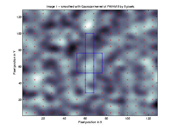
This is best illustrated using a figure. The figure below is based on one of the figures from [wiki:PrinciplesMultipleComparisons my random fields tutorial]. I have taken a set of 128 by 128 independent random numbers, and smoothed them with a kernel of 8 pixels FWHM (see [wiki:PrinciplesSmoothing my smoothing tutorial] for an explanation of this procedure). http://imaging.mrc-cbu.cam.ac.uk/images/svfig.jpg The centre of each resel is marked with a cross. In the centre of the figure is a square with sides that are 24 pixels long. This square, including its edges, contains 4 x 4 = 16 crosses (resel centres). Given that resels are related to independent observations, a larger square will contain more resels, and therefore have more independent observations.
Why shape?
Different shapes will contain data from different numbers of resels. In the figure above, there is also a long thin box, which is of the same volume as the square. This shape abuts on 18 resel centres, so that, even for the same volume, the resel correction will depend on the shape.
How do I use this correction?
Some of the formulae from W96 are implemented in SPM99 and later. They are used to calculate the whole brain random field corrections, and for the output of the SVC (Small Volume Correction) button, in the input window after you have entered the results section. This button will give you p values (expected Euler characteristics) for voxels contained within boxes or spheres centred around the current selected voxel in the results window, or for voxels within a masking image (see the [#DefVVOI Creating VVOI images] section for more details). An image is useful when you have an apriori hypothesis about where the activation is, that is not a box shape or a sphere. We may therefore need to define our search region to be a more complex shape; this shape might correspond to an anatomical region, or the results of an activation from a previous experiment.
Choosing appropriate volumes of interest
The p values given by using the box, sphere or VVOIs are approximate. In particular, for the VVOIs, the approximation is most accurate when the shape is convex, such as an ellipsoid. Complex non-convex shapes, such as an unsmoothed gray matter map, may have a large surface area compared to its volume, leading to higher thresholds than may be appropriate (see W96 for discussion). In addition, VVOIs with curved edges will appear to have a larger surface area than corresponding continuous shapes. This is because the surface area is inflated by the lego-brick effect at the VVOI edges. For this reason, on the suggestion of Keith Worsley, SPM applies a correction to the calculated surface area and diameter of VVOIs, on the basis that most regions specified with VVOIs are likely to have curved edges. When the VVOI has little or no lego-brick effect - for example when the VVOI is a perfect box shape - the surface area correction for VVOIs will not be appropriate, and the "box" specification option is better. Note that the calculations always assume 3D VOIs. Calculations for 2D shapes should be simple to implement given the underlying code.
Creating VVOI images
Images for VVOI calculation need to be the same shape, size and orientation as the region of interest in the statistic image. They must have the same orientation in X Y and Z, in voxel space (.mat files and origin values are ignored). Any voxels in the VVOI image that contain values not exactly equal to zero are taken to be within the VVOI.There are two common reasons to create such VVOI images. The first is that you wish to base your VVOI on a thresholded statistical image that is orthogonal to the statistical map for which you wish to derive corrected p values. You might for example have done an earlier experiment that gave an statistical map showing areas of activation, and want to look only within these areas in your current analysis. In such a case you could use SPM to generate the image, by doing the following: use the results section of SPM to display the first statistical map thresholded as required. For SPM99 and later click on the 'write filtered' button in the input window. SPM asks you for an output filename for the thresholded image. This image will contain the test statistic value in the areas surviving the thresholding, and zeros elsewhere, and you can use this image to define the VVOI.
The second common situation is when you wish to look at some predefined anatomical area or set of areas. To create an image defining these areas you will need to use an image editing package that can write analyze 7.5 format images, such as Analyze itself, or Chris Rorden's freeware [MriCroInformation MRIcro package] for the PC.
To use MRIcro, first download the package from the address above. Choose an anatomical image that is in the same space as your statistical map - for example this might be the SPM T1 MRI template if your images were normalized before you did the statistics. Then follow the steps in the MRIcro tutorial (see MriCroInformation for links) to create a region of interest (ROI) defining your volume on the template. You could use an image based on the ROI you have just defined for your correction. However, a problem that usually arises is that the ROI boundaries are smooth in the two planes that you can see while defining the ROI - usually X and Y - but jagged in the third dimension, due to slight mismatch of the ROI across planes. These jagged edges can make the resulting correction too conservative, so it is usually advisable to smooth the ROI before using it for the W96 correction. To do this in MRIcro, when you have finished defining your ROI, choose the File-Export ROI as smoothed Analyze image. In the dialog box, type a suitable FWHM - say 4 - and use a threshold of 0.25 to make sure all the areas in the ROI get included in the image after smoothing. Set ROI is 1 in the bottom pull-down menu and save. You can use MRIcro to check that this does indeed produce a reasonable definition of your area of interest, and you can overlay the area of interest on the original template if you wish - see the tutorial for details.
You can check that the VVOI covers the regions that you expect using the SpmCheckReg button in SPM99.
Some last technical notes
Note that, for the purposes of the VVOI calculations, the voxel values are taken to represent points in a lattice, rather than touching cubes (see W96). Thus a VVOI cube of 6 x 6 x 6 voxels, with 2 x 2 x 2 mm voxel size, will be calculated to have a 10 x 10 x 10 mm volume. The VVOI image does not have to have the same voxel dimensions or voxel size as the statistic image, only it must be the same shape, size and orientation as the region of interest in the statistic image. Non-zero voxels at the edge of the VVOI image are taken to be at the edge of the VVOI. For example, let us imagine that I wanted to define a cube-shaped VVOI of 12 x 12 x 12 mm (in practice this would not be a good idea, because of the surface area correction applied to VVOIs - see above). My statistic image might be 60 x 70 x 60 voxels (which is irrelevant), with voxel size 2 x 2 x 2 mm. A correct VVOI could be (rather bizarrely) defined by saving an image containing only 13 x 13 x 13 voxels, all non-zero, with 1 x 1 x 1 mm voxel size.
MatthewBrett 29/9/99
Reference
Worsley, K.J., Marrett, S., Neelin, P., Vandal, A.C., Friston, K.J., and Evans, A.C. (1996). [http://www.math.mcgill.ca/~keith/unified/unified.abstract.html A unified statistical approach for determining significant signals in images of cerebral activation]. Human Brain Mapping, 4:58-73.