Design efficiency in FMRI

This page tries to address the question of how to design fMRI experiments that are sensitive to (efficient for) a specific hypothesis (i.e, statistical planned comparison or "contrast"). The properties of the BOLD signal measured by fMRI - particularly its "sluggish" nature - can make the design of efficient experiments difficult to intuit. This page starts with some general advice, before explaining the reasons for this advice from the perspectives of 1) signal-processing, 2) mathematics, 3) correlations between regressors. It is hoped that at least one of these different perspectives will aid your intuitions. It finishes with some common questions that I have come across.

Rik Henson (http://www.mrc-cbu.cam.ac.uk/~rh01), 2005

Any comments/corrections welcomed (a lot is also covered in this SPM book chapter Henson, 2006).

General Advice

Scan for as long as possible.

This advice is of course conditional on the subject being able to perform the task satisfactorily (my experience is that subjects can function satisfactorily and comfortably for between 40-60mins within the MRI environment). Longer is better because the power of a statistical inference depends primarily on the number of degrees of freedom (df), and the df's depend on the number of scans (volumes). One might therefore think that reducing the TR (inter-scan interval) will also increase your power: This is true to a certain extent, though the "effective" df's depend on the temporal autocorrelation of the sampled data (i.e, 100 scans rarely mean 100 independent observations), so there is a limit to the power increase afforded by shorter TRs.

If you are only interested in group results (i.e, extrapolating from a random sample of subjects to a population), then the statistical power normally depends more heavily on the number of subjects than the number of scans per subject. In other words, you are likely to have more power with 100 volumes on 20 subjects, than with 400 volumes on 5 subjects, particularly given that inter-subject variability tends to exceed inter-scan variability. Having said this, there are practical issues, like the preparation time necessary to position the subject in the scanner, that mean that 100 volumes on 20 subjects takes more total time than 400 volumes on 5 subjects. A common strategy is therefore to run several experiments on each subject while they are in the scanner (though of course there is nothing wrong with running a single experiment for as long as possible on each subject).

Keep the subject as busy as possible.

This refers to the idea that "deadtime" - time during which the subject is not engaged in the task of interest - should be minimised. Again, of course, there may psychological limits to the subject's performance (e.g, they may need rests), but apart from this, factors such as the inter-trial interval (ITI) should be kept as short as possible (even within blocks of trials). The only situation where you might want longer ITIs (or blocks of rest) is if you want to measure "baseline". From a cognitive perspective though, baseline is rarely meaningful (see Common Question IV regarding null events below).

Only stop the scanner - i.e, break your experiment into separate sessions - if it is strictly necessary (e.g, to give the subject a respite from the noise). Breaks in scanning 1) disrupt the spin equilibrium (i.e, require extra dummy scans), 2) reduce efficiency of any temporal filtering during analysis (since the data no longer constitute a single timeseries), and 3) introduce potential "session" effects ( McGonigle et al, 2000, though see Smith et al, 2005 ).

Do not contrast trials that are far apart in time.

One problem with fMRI is that there is a lot of low-frequency noise. This has various causes, from aliased biorhythms to gradual changes in physical parameters (e.g, ambient temperature). Thus any "signal" (induced by your experiment) that is low-frequency may be difficult to distinguish from background noise. Many analysis packages high-pass filter fMRI data (i.e, remove low-frequency components). Since contrasts between trials that are far apart in time correspond to low-frequency effects, they can be filtered out.

In SPM, for example, a typical high-pass cutoff is 0.01 Hz, based on the observation that the amplitude as a function of frequency, f, for a subject at rest has a "1/f + white noise" form (see ahead to Fig 8 ), in which amplitude has effectively plateaued for frequencies above approximately 0.01 Hz (the inflection point of the "1/f" and "white" noise components). When summing over frequencies (in a statistical analysis), the removal of frequencies below this cut-off will increase the signal-to-noise ratio (SNR), provided that most of the signal is above this frequency (the model residuals are also more likely to be "white", i.e, have equal amplitude across frequencies, an assumption of most parametric statistics).

In the context of blocked designs, the implication is not to use blocks that are too long. For 2 alternating conditions, for example, block lengths of more than 50s would cause the majority of signal (i.e, that at the fundamental frequency of the square-wave alternation) to be removed with a highpass cutoff of 0.01 Hz. In fact, the optimal block length in an on-off design, regardless of any highpass filtering, is approx 16s (as we will see below). This problem of low-frequency noise also means that one should avoid using many conditions of which the important contrasts only involve a subset (see Common Question III below).

Randomise the order, or SOA, of trials close together in time.

As will be explained below, in order to be sensitive to differences between trials close together in time (e.g, less than 20s), one either 1) uses a fixed ITI but varies the order of different trial-types (conditions), or 2) constrains their order but varies the ITI. Thus a design in which two trials alternate every 4s is very inefficient for detecting the difference between them (as explained below). One could either randomise their order (keeping the ITI fixed at 4s), or vary their ITI (keeping the alternating order). Note that, in this context, blocks can be viewed as runs of trials of the same type, and a blocked design corresponds to a varying-ITI design in which there is bimodal distribution of ITIs: a short ITI corresponding to the ITI within blocks, and a long ITI corresponding to the ITI between the last trial of one block and the first of the next (as elaborated below).

Theoretical Background

First some terminology. An experimental condition consists of a number of "trials" (replications of that condition). The time between the onset of successive trials is the ITI. A trial consists of one or more components. These components may be brief bursts of neural activity (impulses, or "events"), or periods of sustained neural activity ("epochs"). A working memory trial, for example, may consist of stimulus (event), a retention interval (epoch) and a response (event). For consistency with previous literature, the time between the onsets of components will be referred to as the Stimulus Onset Asynchrony (SOA) - even if the components are not stimuli per se - whereas the time between the offset of one component and the onset of the next will be referred to as the Interstimulus Interval (ISI). Events are in fact assumed to have zero duration (i.e, are "delta functions"), so for trials consisting of single events, the SOA=ISI. (For epochs, SOA = SD + ISI, where SD is the stimulus duration). For more information about durations, i.e, events vs. epochs, see Common Question VII.

The BOLD impulse response (IR)

A typical BOLD response to an impulse (brief burst) of neural activity is shown as a function of peristimulus time in Fig 1. The peak response occurs at 4-6s, and is often followed by undershoot from approx 10-30s (at high fields, an initial undershoot around 1s is sometimes observed). The precise shape of the IR does vary across individuals, and across brain regions within an individual, though such variation can usually be captured by 3 dimensions ( Henson et al, 2001 ).

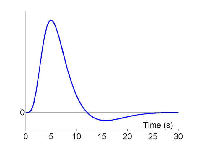
Early event-related fMRI experiments used long SOAs, in order to allow the IR to return to baseline between stimulations. However, this is not necessary if the IRs to successive events summate in linear manner, and in this case, it is generally more efficient, as we shall see below, to use shorter SOAs. One exception is if there are only a limited number of stimuli. In this case, longer SOAs can be more efficient simply because they entail longer scanning sessions, and hence more df's (see General Advice 1 above). The issue of nonlinearities (i.e, saturation at short SOAs) is mentioned later.

Some subsequent fMRI experiments presented stimuli more rapidly, but interspersed them randomly with 'fixation trials' (what are called 'null events' here) and counterbalanced the order of each trial-type. This allows a very simple analysis method (developed in the ERP field) called 'selective averaging' (Dale & Buckner, 1997). However, this analysis method is a special case of more general linear deconvolution methods (that can be implemented within the GLM using temporal basis functions). A 'Finite Impulse Response' (FIR) temporal basis set in SPM, for example, will achieve an identical deconvolution without needing to assume that the order of trial-types is counterbalanced (see Henson, 2006 ).

The arguments below assume an infinite number of scans/trials, though also apply to experiments with reasonable numbers of trials in which randomisation is approximated. They also assume that the basic IR shape is known (so that all that needs to be estimated is its amplitude, i.e, scaling). The latter implies that the contrasts of interest reflect T- or F-tests across conditions using a single assumed IR shape (more precisely, that shown in Fig 1). For hypotheses concerning the shape of the IR (e.g, F-tests spanning several temporal basis functions), see the Common Question V below.

Signal-processing

Given that we can treat fMRI volumes as comprising a timeseries (for each voxel), some intuition can be gained from adopting a signal-processing perspective ( Josephs & Henson, 1999 ). We assume what is called a "linear convolution" model, in which the predicted fMRI series is obtained by convolving a neural function (e.g, stimulus function) with an assumed IR.The concept of convolution is best understood by a series of examples. We consider first the ability to detect the BOLD response to a single event-type versus baseline (we will consider multiple event-types later, in Maths section ). For an event occurring every 16s, the results of convolution using the IR in Fig 1 are shown in Fig 2 (the convolution operator is indicated by the encircled "times" symbol).

The basic idea behind maximising efficiency is to maximise the "energy" of the predicted fMRI timeseries. This is simply the sum of squared signal values at each scan. It is also proportional to the variance of the signal (see later Maths section ). In other words, to be best able to detect the signal in the presence of background noise (not shown), we want to maximise the variability of that signal. A signal that varies little will be difficult to detect.

Now the above example (a fixed SOA of 16s) is not particularly efficient, as we shall see later. What if we present the stimuli much faster, e.g, every 4s? This is shown in Fig 3.

Because the IRs to successive events now overlap considerably, we end up an initial build-up (transient) followed by small oscillations around a "raised baseline". Although the overall signal is high, its variance is low, and the majority of stimulus energy will be lost after highpass filtering (particularly after removal of the mean, i.e lowest frequency). So this is an even less efficient design.

What if we vary the SOA randomly? Let's say we have a minimal SOA of 4s, but only a 50% probability of an event every 4s. This is called a stochastic design (and one way to implement it is simply to randomly intermix an equal number of "null events" with the "true events"). This is shown in Fig 4.

Though we only use half as many stimuli as in Fig 3, this is a more efficient design. This is because there is a much larger variability in the signal (and we know how this signal varies, even though we generated the event sequence randomly, because we know the specific sequence that resulted).

We could also vary the SOA in a more systematic fashion. We could have runs of events, followed by runs of no (null) events. This corresponds to a blocked design. For example, we could have blocks of 5 stimuli presented every 4s, alternating with 20s of rest, as shown in Fig 5.

This is even more efficient than the previous stochastic design. To see why, we shall consider the Fourier transform of these timeseries. Firstly however, note that, with such short SOAs (approx 4s or less), the predicted fMRI timeseries for such a blocked design is very similar to what would obtain if neural activity were sustained throughout the block (i.e, during the ISI as well). This is called an "epoch" in SPM, and would correspond to a square-wave (or "box-car") function, as shown in the top row of Fig 6.

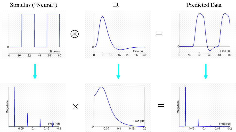
Now if we take the Fourier transform of each function in the top row (after extending the timeseries for much longer), we can plot amplitude (magnitude) as a function of frequency as shown in the bottom row. The amplitude spectra (square-root of the "power spectra") of the square-wave neural function has a dominant frequency corresponding to its "fundamental" frequency (Fo = 1/(20s+20s) = 0.025 Hz), plus a series of "harmonics" (3Fo, 5Fo, ... etc) of progressively decreasing amplitude. The fundamental frequency corresponds to the frequency of a sinusoidal that best matches the basic on-off alternation; the harmonics can be thought of as capturing the "sharper" edges of the square-wave function relative to this fundamental sinusoid.

The Fourier transform does not affect the data or conclusions, so why bother? Well it offers a slightly different perspective. Foremost, a convolution in time is equivalent to a multiplication in frequency space. In this way, we can regard the neural activity as our original data and the IR as a "filter". You can see immediately from the shape of the Fourier transform of the IR (second panel of the bottom row) that this filter will "pass" low frequencies, but attenuate higher frequencies (which is why it is sometimes called a "lowpass filter" or "temporal smoothing kernel"). This property is why, for example, much high-frequency information was lost in the fixed SOA=4s design in Fig 3. In the present epoch example, the result of multiplying the amplitude spectrum of the neural data by that of the filter is that some of the higher-frequency harmonics are attenuated, but the amplitude of the fundamental frequency is attenuated little. In other words, the majority of the signal is "passed" by the IR filter.

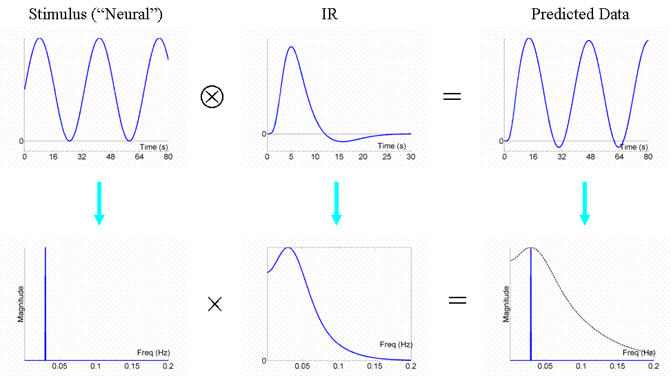
We are now in a position to answer the question: what is the most efficient design of all? Well, assuming we had a limited amount of total "stimulus energy", the optimal design would be to modulate the neural activity in a sinusoidal fashion (e.g, sinusoidally varying the luminance of a visual stimulus), with a frequency that matches the peak of the amplitude spectrum of the IR filter. With the assumed IR shape used here, this would be ~0.03Hz (1/30s). The sinusoidal modulation places all the stimulus energy at this single frequency, shown by the single line in frequency space in Fig 7:

We can now also turn to the question of highpass filtering: the common strategy for dealing with the excessive low-frequency noise in fMRI data, as mentioned above in General Advice 3. fMRI noise tends to have two components: low-frequency "1/f" noise and background "white noise", shown by the dark and light blue lines respectively in Fig 8. The goal of high-pass filtering is to maximise the loss of noise but minimise the loss of signal. A sinusoidal modulation of signal at 0.03Hz is shown in red, for which a highpass cut-off of 0.01Hz would be fine (i.e, removal of the hatched frequencies).

Because the filtering is commutative, we can apply the highpass filter to the lowpass filter inherent in the IR to create a single "band-pass" filter (or "effective HRF", Josephs & Henson, 1999 ). This is shown in Fig 9 below, in which the highpass filter reflects the "chunk" of low-frequencies has been removed from the IR filter (highpass cut-off here = 1/120s ~ 0.008 Hz).

The consequence of highpass filtering is shown for long blocks of 80s (20 trials every 4s). Because the fundamental frequency in this design (1/160s ~ 0.006 Hz) is lower than the highpass cutoff, a large proportion of signal energy is lost (reflected by the rather strange shape of the predicted fMRI timeseries, in which the lowest frequency has been removed). This is therefore not an efficient design (with this specific highpass cut-off). This illustrates the general point that blocked designs are only efficient when the block length is not too long ( General Advice 3 ): approx 16s-on, 16s-off is optimal (with the present IR); block durations of up to 50s-on, 50s-off are also fine (given that the IR filter does not attenuate low-frequencies much); but block durations much longer than this (or contrasts between two of many different types of 50s-blocks, see Common Question III ) may be in danger of being swamped by low-frequency noise.

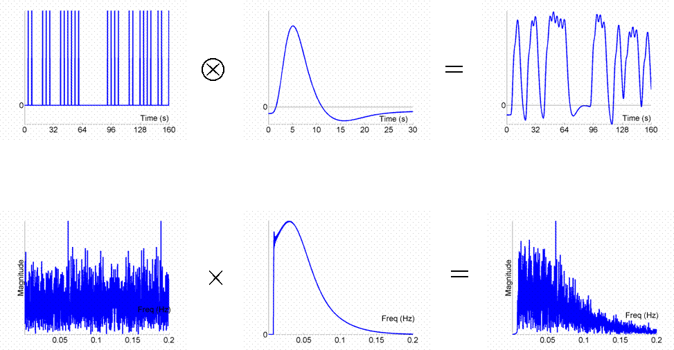
Finally, we can return to consider what happens in a stochastic design like that in Fig 4. The effect of the randomised SOA is to "spread" the signal energy across a range of frequencies, as shown in Fig 10. Some of the high and low frequency components are lost to the effective IR bandpass filter, but much is passed, making it a reasonably efficient design (for the fixed SOA=4s version, much more signal will live at high frequencies - viz multiples of 0.25Hz - and so be lost). This is the rationale for General Advice 4.

Mathematics (statistics)

Within the General Linear Model (GLM), the equation for a T-statistic is:

T = c'*b / sqrt(var( c'*b ))

where c is a column vector of contrast weights (e.g, c= [+1 -1]' to contrast two conditions), b is a column vector of parameter estimates (regression coefficients), the apostrophe symbolises the transpose operator, and var(v) refers to (an estimate of) the variance of v.

Assuming that the error, estimated from the model residuals, is drawn independently for each observation from the same Gaussian distribution ("iid"):

var( c'*b ) = s^2 c'*inv(X'X)*c

where X is the design matrix (model), inv is the matrix inverse, and s^2 is an estimate of the error variance derived from the sum of squares of the residuals. So, in order to maximise our T-values, we need to minimise this quantity. Assuming that the error (noise) is independent of our experimental design (X), and that our planned contrast (c) is fixed, all we can play with is X.

If we are interested in multiple contrasts, we can make C a matrix of contrast weights, which leads to a statistical definition of efficiency, e, as:

e(C,X) = trace( C'*inv(X'X)*C )^-1 [Eqn 1]

Note that e has no units, and is a relative measure. It depends on the scaling of the design matrix and the scaling of the contrasts. It is unlikely to map simply onto real T-values; though we expect it to be at least monotonically related to them. Thus all we can really say is that one design/contrast combination is more efficient than another; we cannot say a design is "twice" as good as another, just because e is twice as big.

If we start with a single event-type (and an assumed IR, as above), such that X has a single column and c=[1] , then we can parameterise any design using only two quantities:

1. T, or "SOAmin", the minimal time between events, and 2. p(t), the probability of an event occurring each t = T, 2T, 3T... etc

A "deterministic" design is one in which p(t)=1. The top row of Fig 11 corresponds to an example of such a "fixed SOA" design with T=8s. The efficiency of this design (plotted from left-to-right) is low (Friston et al, 1999).

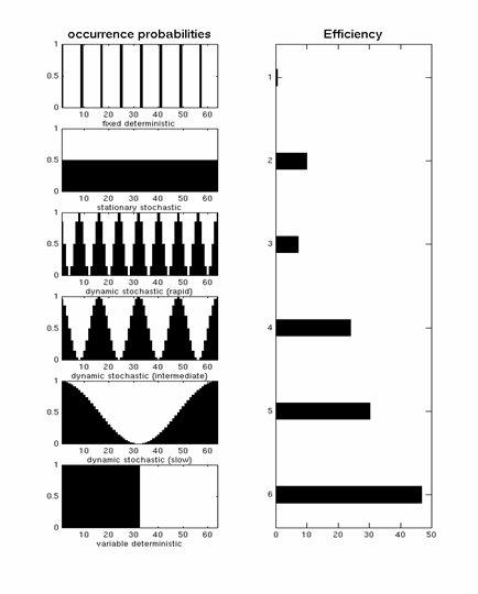
A "stationary stochastic" design is one in which p(t) is less than 1 but constant over time. This corresponds to the second row of Fig 11, and is more efficient (with a shorter SOAmin) than the fixed SOA=8s design.

A "dynamic stochastic" design is one in which p(t) is a function of time. An extreme example of this is a blocked design (bottom row of Fig 11), for which p(t)=1 inside a block, and p(t)=0 outside a block. This is very efficient (as also explained in the signal-processing section). One potential problem with blocked designs however is that the response to events within a block may be confounded by the context of their occurrence, e.g, subjects become aware of the blocking and may alter their strategies/attention as a consequence. The remaining rows in Fig 11 correspond to dynamic stochastic designs in which p(t) is modulated in a sinusoidal fashion. In other words, these designs produce clumps of events close together in time, interspersed with periods in which events are rarer. Though such designs are less efficient than the extreme blocked design, they can be more efficient than a stationary stochastic design (second row of Fig 11), and assuming that subjects are less likely to notice the "clumping" of events, may offer a nice compromise between efficiency and subjective "unpredictability".

What about the situation when we have multiple event-types (conditions)? Firstly, we now have more possible contrasts that might be of interest. If we have 2 event-types for example, we might be interested in the "differential effect" between them (a c= [+1 -1]' contrast) and/or their "common effect" versus the interstimulus baseline (a c= [+1 +1]' contrast). Different contrasts will have different efficiencies (even with the same design matrix).

Secondly, we can still parameterise these designs in terms of SOAmin, as before, but now the probability, p_i(h), of a specific event-type i=1...N occurring every SOAmin can be expressed as a function of the history h, a vector of the previous j=1...M event-types. These probabilities can be captured in terms of a NM x N "transition matrix". This is best illustrated by examples.

A "randomised" design in which two event-types were randomly intermixed would have a first-order (M=1) transition matrix:

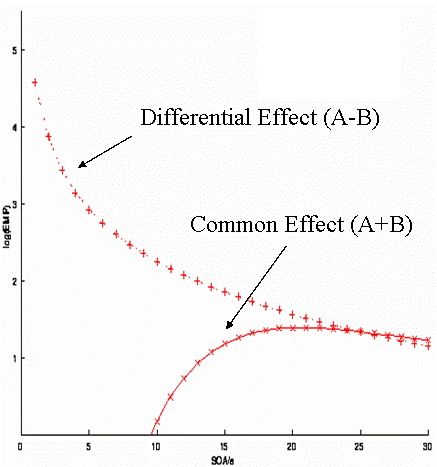
In other words, there is a 50% probability of A or B, regardless of the previous event-type. (This transition matrix is rather redundant, but shown this way in order to compare with subsequent examples.) For this randomised design, the efficiency for both the differential and the common effect is shown in Fig 12. The optimal SOA clearly differs for the two contrasts. For the common effect, the optimal SOA is approx 16-20s; for the differential effect, the optimal SOA is the shortest SOA possible (under the present linear assumptions; the issue of saturation at short SOAs is covered later ).

Imagine another situation, in which A and B must alternate for some reason (e.g, if A and B were two percepts of a bistable stimulus). This would correspond to the simple transition matrix:

The question then becomes what is the optimal SOA for detecting the differential effect? From the blue curve in Fig 13, one can see the answer is 8-10s.

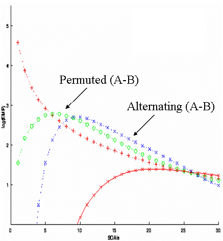Imagine another situation in which the SOA cannot be less than 5s (for whatever reason). Can we do better than a fully-randomised design (red), but without alternating the stimuli? One possibility is to use a "pseudo-randomised" design. This would correspond to the second-order (M=2) transition matrix:

This is randomised to first-order, but fully deterministic to second-order. Its efficiency for detecting the difference between A and B corresponds to the green line in Fig 13. Thus it is better than a fully-randomised design for SOAs more than ~5s. It is less efficient than an alternating design for SOAs of more than ~8s, but has the potential advantage of being less predictable (people are generally poor at detecting higher-order contingencies). Having said this, whenever structure is introduced into sequences, one should beware of potential conscious or unconscious effects of that structure on cognitive processing.

Finally, we can consider the introduction of "null events". These simply correspond to an additional event-type that is randomly intermixed with the event-types of interest. Since null events do not entail any change from whatever comprises the interstimulus interval (e.g, a fixation crosshair), they simply provide a convenient way of randomising the SOA between the events of interest, i.e, of generating a "stochastic" design in the earlier terminology. They correspond to transition matrices in which the rows do not sum to 1. So if we added null-events in equal proportion to our A and B event-types, we would have the transition matrix:

Why add null events? Well, the answer is that they buy us efficiency for detecting the common effect (e.g, of A and/or B vs. interstimulus baseline) even at short SOAs (with a small reduction of efficiency for detecting the differential effect). This is shown in the two green lines in Fig 14.

This may be important if we want to be sensitive to both contrasts. For example, if A and B were happy and sad faces, we may want to ask 1) where in the brain is there a response to faces vs. baseline (regardless of expression, a [+1 +1] contrast) and 2) where, within those regions responsive to faces (i.e, using a mask or functionally-defined ROIs from the first contrast), is there a difference between happy and sad faces (the [+1 -1] contrast)?

Note that random intermixing of null events with events of interest produces an exponentially-decreasing distribution of SOAs (i.e, fewer long than short SOAs). There may be more efficient distributions of SOAs from which to generate event sequences (see, eg, Hagberg et al, 2001 ), and optimal ways of ordering different event-types (e.g, using "m-sequences", Buracas & Boyton, 2002 ).

Impact of nonlinearities on efficiency

The above efficiency arguments have assumed linearity, i.e, that the responses to successive responses summate linearly, no matter how close together they are. In reality, we know there is a "saturation", or under-additivity, even for SOAs of ~10s. This means that the efficiency curves shown in the figures above cannot increase indefinitely as the SOA decreases. The saturation could have neural and/or haemodynamic causes. However, the size of this nonlinearity appears to be relatively small until SOAs of a few seconds are reached: By estimating the nonlinearity (in a particular brain area in a particular design), Friston et al (1999) calculated the impact of such nonlinearities on the predicted efficiency. The result is shown in Fig 15.

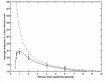The dotted line shows efficiency under linear assumptions; the solid line shows the effects of saturation. While the solid line is below the dotted line for all SOAs (below 10s), the divergence is small until SOAs of 1-2s. Indeed, the predictions of this calculation is that the optimal SOA can be as low as 1s. It should be noted that this prediction is based on a specific dataset, and may not generalise, but it suggests that the advantage of short SOAs can outweigh the saturation of responses until surprisingly short SOAs. (Note however that the appreciable saturation at such short SOAs also implies that such nonlinearities should be included in the statistical model, e.g, via a linearisation using Volterra kernels, Friston et al, 1999, to avoid systematic error in the residuals.)

Correlation between regressors

Another way of thinking about efficiency is to think in terms of the correlation between (contrasts of) regressors within the design matrix. If we consider Equation [1] above, the term X'X reflects the covariance of the design matrix, X. High covariance (correlation) between the columns of X increases the elements in inv(X'X), which can decrease efficiency (depending on the particular contrast, C).

Let's consider the earlier example of two event-types, A and B, randomly intermixed, with a short SOA. If we plot the resulting two regressors (after convolution with an assumed IR) against each other, we would end up with a scatter plot something like that in Fig 16. The high negative correlation between the regressors is because whenever there is high signal for A, there tends to be low signal for B, and vice versa.

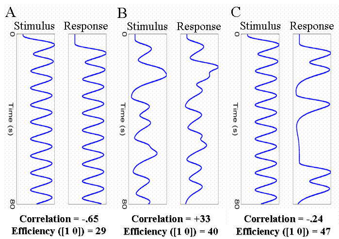
If we consider the projection of this 2D distribution onto the x=-y direction (corresponding to a [1 -1] contrast), it will have a large spread, i.e, high variance, which means that we will be efficient for detecting the difference between A and B in this design. However, if we project the distribution onto the x=y direction (corresponding to a [+1 +1] contrast), it will have little spread, i.e, low variance, which means that we will not be efficient for detecting the common effect of A and B versus baseline. This corresponds to the markedly different efficiency for these two contrasts at short SOAs that was shown in Fig 12. Likewise, projection onto the x or y axes ( [1 0] or [0 1] contrasts) will have less spread than onto the x=-y direction (and less than if the two regressors were uncorrelated (orthogonal), which would correspond to a spherical cloud of points, with the same "radius" as along the x=-y direction in the present example).

This example also makes an important general point about correlations. High correlation between two regressors means that the parameter estimate for each one will be estimated inefficiently, i.e, the parameter estimate itself will have high variance. In other words, if we estimated each parameter many times (with different random noise) we would get wildly different results. In the extreme case that the regressors are perfectly correlated (correlation of +/-1, ie, collinear), we could not estimate unique values for their parameters (ie, they would have infinite variance). Nonetheless, we could still estimate efficiently the difference between them. Thus in short-SOA, randomised designs with no null events, we might detect brain regions showing a reliable difference between event-types, yet when we plot the event-related response, we might find they are all "activations" vs. baseline, all "deactivations" vs. baseline or some activations and some deactivations. However, these impressions are more apparent than real (and should not really be shown): If we tested the reliability of these activations / deactivations, they are unlikely to be significant. This is again because there is high variability associated with each estimate on its own, even if there is low variability for the estimate of the difference. In other words, we cannot estimate baseline reliably in such designs. This is why, for such designs, it does not make sense to plot error bars showing the variability of each condition alone: one should plot error bars pertaining to the variability of the difference.

Another common misapprehension is that one can overcome the problem of correlated regressors by "orthogonalising" one regressor with respect to the other. This rarely solves the problem. The parameter estimates ALWAYS pertain to the orthogonal part of each regressor (this is an automatic property of mean-square fits within the GLM). Thus the parameter estimate (and its variance) for the orthogonalised regressor will NOT change. The parameter estimate for the other regressor will change, and will be estimated more efficiently. However, this parameter estimate now reflects the assumption that the common variance is uniquely attributed to this regressor. We must have an a priori reason for assuming this (ie, without such prior knowledge, there is no way to determine which of the two correlated regressors caused the common effect). In the absence of such knowledge, there is no need to orthogonalise.

Anyway, returning to the effects of correlations on efficiency, this conception can help with the design of experiments where there is necessarily some degree of correlation between regressors. Two main experimental situations where this arises are: 1) when trials consist of two events, one of which must follow the other, and 2) blocks of events in which one wishes to distinguish transient (event-related) from sustained (epoch-related) effects.

A common example of the first type of experiment are "working memory" designs, in which a trial consists of a stimulus, a short retention interval, and then a response. We shall ignore the retention interval, and concentrate on how one can estimate separate effects of the stimulus and of the response. With short SOAs between each event-type (eg, 4s), the regressors for the stimulus and response will be negatively correlated, as shown in Fig 17(A).

Two possible solutions to this problem are shown in Fig 17(B) and 17(C). The first is to randomly vary (jitter) the time between successive stimuli and responses (assuming this is possible). The second is to keep the stimulus-response interval fixed at 4s, but only require a response on a random half of trials. The effect of both is to reduce the correlation between the regressors, which increases the efficiency for separating the brain's activity to stimuli and to responses. Note that the first solution - jittering the stimulus-response and response-stimulus intervals - does require jittering over quite a large range, in order to reduce the correlation appreciably.

The second type of experiment, which has become popular recently, tries to distinguish transient responses (or so-called "item" effects) from sustained responses (or so-called "state" effects). A lovely example of this is the experiment on visual attention by Chawla et al, 1999, in which the authors showed that attention to motion or colour of moving dots had two effects: it increased both the baseline activity (a "state" effect) and the gain of responses to a change in the attended attribute (an "item" effect). This was true for colour in V4, and for motion in V5. Such separation of transient and sustained effects requires modelling blocks of trials in terms of both individual events within blocks and sustained epochs throughout the blocks. An example with a fixed SOA=4s between events is shown in Fig 18(A).

With a fixed SOA of 4s, as in Fig 18(A), the correlation between the event and epoch regressors is naturally very high, and the efficiency for detecting either effect alone is low. Using the same total number of events per block, but with a pseudorandomised design in which the events are randomly spread over the block with a minimal SOA of 2s (Fig 18(B)), the correlation is reduced and efficiency increased. (Note that one perverse consequence of having to introduce some long SOAs between events within blocks in such so-called "mixed designs" is that subjects may be less able to maintain a specific cognitive "state".)

This concludes these three attempts to explain the basic ideas behind efficiency in fMRI designs. I hope at least one perspective helped. Below are a collection of various related questions that are often raised.

Common Questions

I. What is the minimum number of events I need?

Unfortunately, there is no answer to this, other than "the more, the better". The statistical power depends on the effect size and variability, and this is normally unknown. People who say "you cannot do an event-related fMRI analysis with less than N events" are talking rubbish, unless they have a specific effect size in mind (which is a function of the experimental effect, the brain region, the scanner strength, the sequence optimization, etc, etc...). Note it is even possible that fewer trials are required (for a given power) than for an equivalent contrast of behavioural data (the noise in, e.g, response times (RTs) may exceed that in a specific cortical region contributing to those RTs). Furthermore, it is not even the number of events per se that is relevant: it is also the SOA and event-ordering (see next question).

II. Doesn't shorter SOAs mean more power simply because of more trials?

It is not simply the number of trials: the temporal distribution of those trials is vital (as explained above). Thus 400 stimuli every 3s is LESS efficient than 40 stimuli every 30s for detecting a single event-related response versus interstimulus baseline (since a fixed SOA of 3s produces little experimental variability after convolution by the IR; see Fig 3 ). 200 stimuli occurring with a 50% probably every 3s (i.e, pseudorandomly mixed with 200 null events) is much more efficient than either. Note again, as mentioned above, if you have a limited number of trials (eg stimuli), but plenty of scan time, long SOAs can be more efficient than short SOAs by virtue of allowing more volumes to be acquired in total (ie longer experiment, ie more df's). The efficiency arguments above are predicted on having a fixed scan time, over which an effectively unlimited number of trials can be distributed (eg a sufficiently large stimulus set).

III. What is the maximum number of conditions I can have?

A common interpretation of General Advice 3 above - not to contrast trials that are too far apart in time - is not to design experiments with too many experimental conditions. More conditions necessarily mean that replications of a particular condition will be further apart in time. However, the critical factor is not the number of conditions per se, but the specific contrasts performed over those conditions. For pairwise comparisons of only 2 of, say, 8 blocked conditions (e.g, a [1 -1 0 0 0 0 0 0] contrast), the above caveat would apply: if there were equal numbers of blocks of each condition, blocks longer than 12.5s (100s/8) are likely to entail a substantial loss of signal when using a highpass cutoff of 0.01Hz. However, this caveat would not apply if the contrasts of interest included ("spanned") all 8 conditions, as would be the case if the experimenter were only interested in the two main effects and the interaction within a 2x4 factorial design (i.e, contrasts like [1 1 1 1 -1 -1 -1 -1] ). If you must compare or plot only a subset of many such blocked conditions, you should consider presenting those blocks in a fixed order, rather than random or counter-balanced order, which will minimise the time between replications of each condition, i.e, maximise the frequency of the contrast.

IV. Should I use null events?

Null events are simply a convenient means of achieving a stochastic distribution of SOAs, in order to allow estimation of the response vs. interstimulus baseline, by randomly intermixing them with the events of interest. However, the "baseline" may not always be meaningful. It may be well-defined for V1, in terms of visual flashs versus a dark background. It becomes less well-defined for "higher" regions associated with cognition however, because it is often unclear what these regions are "doing" during the interstimulus interval. The experimenter normally has little control over this. Also note that the baseline is only as good as it controls for differences relative to the events of interest (e.g, a fixation cross hair does not control for visual size when used as a baseline for words). Moreover, it does not control for the fact that the events are impulsive (rapid changes) whereas the baseline is sustained (and may entail, e.g, adaptation or reduced attention). For this reason, it is often better to forget about baseline and add an extra low-level control event instead.

Another problem with null events is that, if they are too rare (e.g, less than approx 33%), they actually become "true" events in the sense that subjects may be expecting an event at the next SOAmin and so be surprised when it does not occur (the so-called "missing stimulus" effect that is well-known in ERP research). One solution is to replace randomly intermixed null events with periods of baseline between blocks of events. This will increase the efficiency for detecting the common effect vs. baseline, at a slight cost in efficiency for detecting differences between the randomised event-types within each block.

Yet another problem is that sometimes the unpredictability of the occurrence of true events (caused by the randomly intermixed null events) can cause delayed or even missed processing of the events of interest. If subjects must respond quickly to each event, for example, it is often advantageous if they know roughly when each event will occur, and so prepare for it.

So to answer the question, null events are probably only worthwhile if 1) you think the mean activity during the constant interstimulus interval is meaningful to contrast against, 2) you don't mind null events being reasonably frequent (to avoid "missing stimulus" effects) and 3) you don't mind the stimulus occurrence being unpredictable (as far as the subject is concerned). Having said this, some form of baseline can often serve as a useful "safety net" (e.g, if you fail to detect differences between two visual event-types of interest, you can at least examine V1 responses and check that you are seeing a basic evoked response to both event-types - if not, you can question the quality of your data or accuracy of your model). But then again, that baseline might be better estimated from "blocked" periods of baseline, rather than randomly intermixed null events.

Remember that randomly intermixed null events are not NECESSARY to analyse event-related responses if you have a rough idea what form the BOLD impulse response takes (see above ). If however you do want to estimate the precise shape of the BOLD impulse response, then they do become necessary, as detailed in the next question:

V. What is the difference between 'detection power' and 'estimation efficiency' ?

Liu et al, 2001 and others have pointed out that designs have different efficiencies for 1) detecting a difference in the amplitude of an assumed IR, and 2) characterising the shape of the IR. Blocked designs are normally most efficient for the former, and stationary stochastic designs are most efficient for the latter. All arguments above are restricted to the former, since we are normally interested in estimating the size of an IR, rather than its precise shape. This distinction actually reduces to the choice of temporal basis functions. So the same efficiency Equation [1] above can be used to optimise either detection power or estimation efficiency simply by using different response functions: e.g, either a canonical HRF or an FIR basis set respectively in SPM (see Henson, 2004 for further explanation).

VI. Should I generate multiple random designs and choose the most efficient one ?

This is certainly possible, though be wary that such designs are likely to converge on designs with some structure (e.g, blocked designs, given that they tend to be optimal, as explained above). This may be problematic if such structure affects subjects' behaviour (particularly if they notice the structure). Note however that there are software tools available that optimise designs at the same time as allowing users to specify a certain level of counterbalancing (to avoid fully blocked designs): e.g, Wager & Nichols, 2003, or the OptSeq program developed by Doug Greve.

VII. Should I treat my trials as events or epochs ?

Trials - e.g, presentation of a stimulus followed by a behavioural response - clearly have a finite duration. If all trials were of the same duration however, and that duration were below ~2s, then they can be effectively modelled as events (i.e, delta functions with zero duration). This is because, after convolution with the IR, a difference in the duration of a trial causes a difference in the scaling (size) of the predicted response, but has little effect on its shape (see Fig 19 below). Since it is the scaling of the predicted response that is being estimated in the statistical models discussed above, changing the duration of all trials (from 0-2s) simply changes the size of the resulting parameter estimates, with little effect on the statistical inferences (given typical SNRs). This is despite the fact that the efficiency, as calculated by Equation [1], will increase with longer durations (ie, with greater scaling of the regressors in the model,X). This increase is correct, in the sense that a larger signal will be easier to detect in the presence of the same noise, but misleading in the sense that it is the size of the signal that we are estimating with our model (i.e, the data themselves are unaffected by how we model the trials). For longer duration trials, the response begins to plateau, meaning that an "epoch model" can be a better model. More important however, is the case of trials that vary in duration from trial to trial within a condition, or across conditions. Whether these are better modelled as events, or as epochs of different durations (e.g, with duration equal to the RT for each trial), is debatable. For example, if the stimulus duration were constant and only RTs varied, then the activity in V1 may not be expected to vary with RT, so an "event model" might fit better (and in this case, the parameter estimate can be interpreted as the BOLD response per trial). For activity in premotor cortex on the other hand, greater activity might be expected for trials with longer RTs, so a "varying-epoch model" might fit better (and in this case, the parameter estimate can be interpreted as the BOLD response per unit time). So the answer depends on your assumptions about the duration of neural activity in the particular brain regions of interest.

Acknowledgements

Thanks to Ged Ridgway, Daniel Bor and Floris de Lange for their helpful comments, and Matthew Brett for WIKIfying.