
FMRI analysis defaults
This page describes the default analysis steps for WBIC data. These are data collected before June 2006 on the WBIC Bruker 3T scanner.
The description here is of the steps you will need to take in the GUI to analyze in SPM, with some discussion of the AnalysisPrinciples involved. Personally (MatthewBrett) I would recommend that someone new to imaging, or new to SPM, does a few analyses this way to get themselves used to the interface and the processing steps involved.
After a few runs of this you will start to thirst after some more automated system. You can try the various batch examples (SpmBatch2, SpmBatch5), or use Rhodri's AA system.
All the preprocessing steps (from data retrieval to smoothing) can now be carried out automatically, via [wiki:AutomaticAnalysisIntroduction Rhodri Cusacks AA scripts]. It is highly recommended that you preprocess using this method when you are used to the analysis.
If you want to read this page on a printed copy, I suggest you also print:
(Bruker data) [wiki:BrukerDataLocation Getting WBIC data] page
(Bruker data) [wiki:FormatBruker Bruker format] page
(Bruker data) [http://pvconv.sourceforge.net pvconv] page
- [wiki:Ana4Dto3D ana4dto3d] page
[wiki:FormatSpmAnalyze SPM Analyze image format]
Identifying the [wiki:FindingCommissures cerebral commissures]
[wiki:MaskedEpiNormalization Masked EPI normalization]
You will get useful additional information from the [http://www.fil.ion.ucl.ac.uk/spm/course/manual/man.htm SPM99 manual], [http://www-psych.stanford.edu/~kalina/SPM99/Protocols/spm99_prepros_prot.html Kalina Christoff's preprocessing webpages] (which don't precisely apply to our data, but are very well explained), and from searching the [http://www.jiscmail.ac.uk/lists/spm.shtml SPM mailing list archives] for specific topics, such as "slice timing" etc.
A) Non-SPM Preprocessing - moving from raw data to SPM images
There are various steps required to convert the raw data once it has arrived at the CBU to images that SPM will apply preprocessing steps on. Initially, if the data have been acquired on the new standard EPI protocols (for instance, those with a 1.1s or 1.6s TR), then we also need to reconstruct the data ourselves. Following this, the reconstructed data need to be converted to Analyze format, so that SPM can read the images. Finally, the 4D Analyze images created need to be split into 3D images (without a time component per image).
Each of these stages can be accomplished by in house software at the command prompt (see below). However, there is a useful program that creates a batch file to automatically perform all the stages above (or a subset of these as the need arises), as well as a few other common steps carried out at this stage (writing appropriate directories out to place the different types of files, copy phase maps and structural images to useful locations, etc.). See [http://www.mrc-cbu.cam.ac.uk/personal/daniel.bor/makefmribatch/ Daniel Bor's MakefMRIBatch page] for details about how to run this program and the batch file it generates.
Getting the data
If you have Bruker data from the Wolfson Brain Imaging Centre, see the [wiki:BrukerDataLocation Bruker data page]. If you followed the steps in these pages, you should now have 4D (X,Y,Z, time) [wiki:FormatAnalyze Analyze format] images for the functional runs, and 3D images for the structural etc scans.
Making images for SPM
There are two steps needed before processing the data with SPM; you will need to convert the 4D functional images into a series 3D volumes, with one volume for each time point. Then you may need to discard a few dummy scans from the beginning of the time series. Deleting dummy scans is useful because there is a large signal change in the first few images in a functional dataset, as the tissue reaches a steady state of radiofrequency excitation. We usually discard 15 seconds of data (5 scans with a TR of 3, 8 scans with a TR of 2).You can make the 3D volumes and discard the dummies with the [wiki:Ana4Dto3D ana4dto3d] program. If you do not use ana4dto3d to throw away the dummies, and you are going to discard the first few images, now would be a good time to move them out of the directory with the other images, or delete them if you are brave.
Diagnostics
If you have used ana4dto3d, you might have created a mean and variance image for the functional runs. It is a good idea to inspect these using SPM or MriCro, to look for reconstruction or data acquisition problems (funny brain shape, strange effects on lower image slices, high ghost variance, radiofrequency artefact). See the [wiki:DataDiagnostics FMRI diagnostics] page for details.
Now, you can start SPM 99 / SPM2...
B) SPM Preprocessing - from SPM-based raw data to smoothed data ready for analysis
After creating 3D Analyze format images, a number of corrective steps need to be applied before statistical models can be applied:
Slice Timing
See SliceTiming for a discussion of this topic.
First choose "Slice timing" which corrects for different slices of the volume being collected at slightly different times. The MRI scanner at the WBIC performs "interleaved" echo-planar images, to reduce the effect adjacent slices have on each other. First the odd slices are collected, then the even ones. In the slice timing prompts, first select the images in the order they were acquired. In the CBU, we have edited the slice timing routine to add an option to the ensuing list box that is correct for WBIC data; this will be called 'Interleaved (1 3 .. 2 4 ..). Select this option if it is there. If not, choose "user specified" from the menu. Assuming 40 slices, typing "1:2:39 2:2:40" in the text input box, and pressing return will step from 1 to 39 in steps of 2 and from 2 to 40 in steps of 2, giving the order in which the slices were collected. Choose 1 as reference slice (see SliceTimingRikEmail), type in the TR, and the TA. The TA is the Time of Acquisition. Somewhat counterintuitively, the TA is taken as the time between the start of the first slice acquisition, and the start of the acquisition of the last slice. Thus, the default TA, which assumes there is no gap at the end of the volume acquisition, is the TR - TR/(number of slices in the volume). WBIC EPI scans have a gap between the end of the acquisition of the last slice and the beginning of the acquisition of the first slice of the next volume. You need to know what this gap was for your scans. The actual time to acquire one slice is the best value to use to give the TA value (mutliply the slice acquisition time by [no of slices-1] ). The actual slice acquisition time for a Bruker / WBIC image is given in the [wiki:FormatBruker Bruker] text files; getting the repetition times is different for the Bruker sequences (as used by default until early 2002) and Christian's EPI sequences (as used by default since then).
- For the Bruker sequences, you will have an 'imnd' file, in the session subdirectory of the raw data directory. If you have used pvconv to convert your data, the text files will all have been saved with the converted image, as a file "image.brkhdr", where "image.img" is the image file name. The value you want is from the field
##EPI_slice_rep_time
- which gives the time taken to acquire one slice in milliseconds. Thus, if EPI_slice_rep_time = 115, and you have 20 slices, the TA needs to be 0.115 * 19.
- For Christian's EPI sequence, it is a little more complicated; if "srt" is the slice repetition time:
If ##CBU_SliceTiming = Uniform (this is the default): srt = (##PVM_RepetitionTime - ##CBU_TriggerPulseLength) / ##PVM_SPackArrNSlices
If ##CBU_SliceTiming = Bunched; srt = ##PVM_MinRepetitionTime / ##PVM_SPackArrNSlices
Now you need to wait for a bit. The slice timing corrected images have the same name as the originals, but with an "a" prepended to the file name. NB This scheme may well not be correct for FMRI data acquired from other imaging centres - please ask for details.
Image orientation and headers
You may want to reorient your images before you continue the analysis. This has two advantages; first, if you do any analysis on the data from this subject without spatially normalizing, and you have oriented your images roughly to the orientation that SPM expects, then the results will be approximately correctly displayed on the SPM glass or cartoon brain displays. Second, this will give the SPM spatial normalization a good place to start from, and will therefore be less prone to error. The orientation for these purposes does not need to be very accuratem so a few millimetres error will not be important. The orientation you are trying to achieve is shown in the page describing the [wiki:FindingCommissures cerebral commissures]. You may want to keep the images on this page displayed somewhere for reference.In this section we will be creating or modifying .mat files to reorient the images. Another approach is to edit the origin field in the headers (.hdr files) of the [wiki:FormatAnalyze Analyze format] images. I suggest you avoid this, as the origin field is much less flexible than the .mat file, and because the origin field is ignored by SPM when the image has a .mat file, which can cause confusion.
Now, click the display button, and choose the first image in the series, of the slice timing corrected - a*img images.
If you have used a recent version of [http://pvconv.sourceforge.net pvconv] to convert your WBIC ( [wiki:FormatBruker Bruker] )data, you will already have [wiki:FormatSpmAnalyze#matfile .mat files] for your images, which will have oriented the data to neurological (L=L) convention according to the position of the patient in the scanner. If you didn't use the new version of pvconv, or you have deleted the .mat files for the images, and you have saved the Bruker text files, you can recreate the appropriate .mat files using [ttp://pvconv.sourceforge.net brk2mat.pl]. If you have used pvconv therefore, the orientation will be approximately correct when you start (if the subject's head was positioned normally).
If you haven't used pvconv, then your images will probably need some major reorientation in order get them near to the correct neurological orientation. Flip as desired, using the X/Y/Z zooms. For most current EPI images from the WBIC acquired in axial sections (standard) the images will need to be flipped left-right (X) and front-back (Y) to conform to neurological orientation. Do this by applying a -1 resize (zoom) in X and Y in the parameter boxes. On current WBIC images a small bright spot (a bottle of water) can sometimes be seen on the right hand side of the images. Now you have the orientation more or less right, you may want to tume it to better match the orientation of the SPM template. Try comparing your images to the T2 template on the [wiki:FindingCommissures cerebral commissures] page. Start by setting any yaw needed (Z rotation, shaking head type movements), then set roll (Y rotation, moving head to touch ear on shoulder), and pitch (X rotation, nodding). Then use the X Y Z translation boxes to set the blue lines to cross at the anterior commissure.
Don't click on the images during this process, as you will move the blue lines, to some arbitrary point. If you need to reset the blue lines to the current origin, type 0 0 0 in the mm coordinates box in the box on the left of the graphics window, or click on the little embossed line above the coordinate entry boxes.
When you have set all the zooms, rotations and translations to your liking and not before, record the values you are using somewhere for further reference, and then choose "Reorient images" at the bottom of the graphics window. Select all the images in the slice timing corrected - a*img series. If you have used pvconv to convert the data, also select any other images for this subject collected in the same session, as these will be roughly coregistered. When you select Done, this will apply the affine transformations that you have just designed, by adding to, or creating .mat files for all the images.
Check the transformation was as you expected by clicking on "Display" again, and selecting the first image in the slice timing corrected series. The blue lines should cross at the AC, and the image should be in the correct orientation.
Realignment of subject motion
See the MotionCorrection analysis page. If you are following the recipe on this page, you will want to motion correct the slice-time corrected images.
EPI undistortion
EPI images at 3T (e.g. from the WBIC or Oxford) are distorted relative to the structural scans. In order to be able to coregister the EPI images to the structural images properly, we need to first undistort the EPI images to better match the structural in shape. There may be advantages to doing this even if you do not want to coregister to the structural; see [wiki:FmBackground Rhodri's undistortion pages].
Coregistration
See ProcessingCoregistration. Note that, if you have used [http://pvconv.sourceforge.net pvconv] to convert your images from Bruker format, images in the same scanner session should already be coregistered using the automatically generated .mat files from the scanner orientation information.
Normalisation
Time to warp. There are two possible ways to do this. The first is to use the functional mean image and warp it directly to the SPM EPI template. This works well, if you use cost function masking to remove the effects of the susceptibility artefact holes in the EPI images; see the [wiki:MaskedEpiNormalization masked EPI to EPI normalization] page.The second technique is to use the structural image to calculate the normalization, and apply the calculated warping to the functional images. This relies on having good matching between the structural and functional images, and practically this means you will have to use undistortion.
Our current standard practice is to use [wiki:NormalizeSkullStripped the skull-stipped structural image for normalization], after running undistortion on the EPI images with [wiki:FmBackground undistortion toolbox]. This is probably not optimal, and we should probably be normalizing grey matter images, according to the optimized VBM protocol. Sometime soon maybe.
Smoothing
Choose your favourite [wiki:PrinciplesSmoothing smoothing]. Say 8mm for starters. Click on "Smooth", type in the smoothing in mm (here just "8"), select thenormalised - wa*images, wait. Note that SPM2 saves the normalized images with a "w" prefix, where SPM99 used a prefix of "n".
Statistics
When you are familiar with the SPM2 statistics interface, you might consider using [wiki:SpmBatch2 SPM2 batch mode] for statistics, as the model setup is GUI intensive and prone to error.
An example dataset
In the following example, we will set up the model for one session from the [https://sourceforge.net/project/showfiles.php?group_id=76381&package_id=88528 MarsBaR example dataset]. This is a simple one-condition, one-session event-related design - see the [http://marsbar.sourceforge.net/marsbar_devel_tutorial.pdf MarsBaR tutorial], and the README file in the dataset archive for more detail. Here we will analyze session 3 of that dataset. To follow this example, you may want to download and unpack the data archive somewhere, and run the "run_preprocess" script in the "batch" directory in the archive; again, the [http://marsbar.sourceforge.net/marsbar_devel_tutorial.pdf MarsBaR tutorial] lists these steps in more detail. Next you may want to make a new directory to store your example SPM analysis. Change to this directory in matlab ("cd my_directory" or click on the SPM "Utils" menu, and choose "CD" to browse to a directory with the GUI).You should also have a look at the various [http://www.fil.ion.ucl.ac.uk/spm/data/#fMRI_MoAEpilot example datasets] available on the SPM FIL pages.
Specifying the design
To run the GUI, click on the fMRI button in the SPM2 buttons window. http://imaging.mrc-cbu.cam.ac.uk/images/spm2_buttons.png
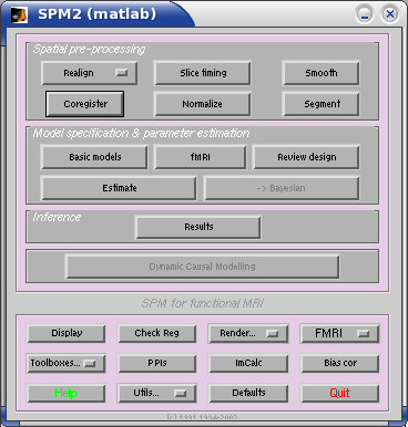
At the prompt "specify design or data", select "design". Give 2.03 as the interscan interval, and 126 as the scans per session. Note that, if we had been analysing - say - three sessions, the entry might have been "126 126 126". Next choose to specify the design in scans rather than seconds. It just so happens that the onset file that I have is in TRs, but of course your onsets could be in seconds from the beginning of the scan run, in which case you would have chosen "seconds" here.
Basis set
Choose: hrf (with time derivative). The basis set is the set of functions that can be used to model your events or blocks. More complex basis sets use more degrees of freedom, can be confusing to review, and may well be better at capturing differences in shape of response between events, or from an assumed HRF shape. Note that, unlike SPM99, you are forced to choose the same basis set for all the events in your model. This design involves a simple visual response, which I expect to be more-or-less the same shape as the standard HRF, so I suggest you choose "hrf (with time derivative)" as a basis set here.
Model interactions (Volterror)
No, no, a thousand times no.
Number of conditions/trials
Choose 1 - we only have one event-type.
Name for condition/trial 1?
Enter: Flashing checkerboard
Vector of onsets
for "Flashing checkerboard". We need to enter the onset times, in TRs (because we chose TR units above), of the flashing checkerboard events. The beginning of the first TR is 0. Here are the event onsets as they should be typed into the entry box:
1.0 9.6 10.2 13.7 22.0 24.0 25.2 30.7 38.2 46.3 47.8 51.6 52.8 58.6 59.9 63.9 79.6
You can copy and paste these out of the browser window, to save time.
Duration(s) (events=0)
The default event duration for SPM2 is "0" - which will actually be converted to an assumed event duration of about 1 second. If each event has a different duration, you will have to enter one value here for each onset, but our events are all the same duration, and the default duration is OK, so enter a single 0.SPM2 does not distinguish events and blocks in its modelling; a block is simply an event with a long duration.
Parametric modulation
Choose: None. This option allows you to model the fact that different events may have different weights; for example you could imagine an experiment where the flashing checkerboard had been of different intensities for different events. This option allows you to enter a weight for each event to take this into into account, but that is not the case here.
User specified [regressors]
Choose: 0. Here you can enter any more regressors for this session. The most common use of this option is to enter the movement parameters into the model, to try and soak up residual movement-related variance. To do this, you could click on "1" (= 1 block of regressors) and then, when asked for values for regressor 1, type "spm_load" in the input box. This allows you to select the rp_*.txt file for this session, and return the values in the file as the regressors. SPM works out that there are in fact 6 regressors, and asks you to name these (say "translation x", "translation y" etc). For simplicity we are not doing that for this model.After all this is done, you will have a new "SPM.mat" file in your matlab current directory, containing the design.
Adding data to the design
Now you have configured the design, you need to specify the scans to use with the design. Click on the "fMRI" button again. This time, select "data" to specify. Next select the "SPM.mat" file you have just created. Next, select the 126 scans for the design; navigate to the "sess3" directory in the example dataset, and select the "snura_sess3_0*img" files. (If you can't see these files, maybe you have not run the "run_preprocess" batch script from the MarsBaR dataset?)
Remove Global effects
Choose: none. This give you the option of using proportional scaling on your data. This will have the effect of dividing all the voxel values for each scan by the thresholded mean voxel value for that scan, so the voxel values are now a ratio of their mean; see the [wiki:PrinciplesStatistics SPM statistics tutorial] for more details. This option can be useful in scanners with significant fluctuations in signal over the course of the scanning session - and specifically, fluctuations that are of higher frequency than your high-pass filter (see below). The disadvantage is this can lead to odd effects if the global signal in the scans has been affected by the activation signal. See Kalina Christoff's [http://www-psych.stanford.edu/~gablab/internal/SPM99/TheoryOfOperation/GlobalScaling.html global scaling page] for more details. The Bruker scanner seems to have fairly good signal stability, and we generally do not use proportional scaling for our data. Some people have found that global scaling is more useful for Oxford data.
High-pass filter
Choose: specify; 128. Here we enter the wavelength in seconds for the high-pass filter. The high-pass filter passes high frequencies, but eliminates low frequencies. FMRI data has a very disproportionate amount of noise at low frequency, and most FMRI designs have small amounts of low frequency components in them, so it is efficient to remove the low frequencies entirely with a high-pass filter. In fact, the SPM2 autocorrelation options more-or-less require that you have a high-pass filter, because they can only model a very limited range of autocorrelation, and this range is suitable for FMRI time-courses after high-pass filtering. The choice of high-pass filter is rather difficult. One way is to look at the design and the data frequency power spectra to see if there is a cut-off that eliminates much of the noise while leaving almost all of the model frequencies. MarsBaR has a tool to do this in an ROI, for example. Here I suggest you accept the default, which captures much of the worst noise. Note that SPM2 does not attempt to match the suggested high-pass cutoff to your design, as was the case for SPM99.
Correct for serial correlations
Choose: AR(1). If you select this option, SPM will attempt to estimate the autocorrelation in the data, and adjust for it - by so-called "whitening" of the time course. This step is necessary if we want to be able to interpret our fixed-effect (e.g single-subject) p values. Because FMRI data with a short TR (as here) have some autocorrelation, we have to take this into account in calculating the statistics. SPM does this using a two-pass procedure. First it estimates the model without taking account the autocorrelation. In the process, it selects out all voxels having a large amount of variance explained by the design (in fact, by the effects of interest). It then pools the covariance of all these "activated" voxels, and estimates a best-fit model of their autocovariance, using a very constrained model. By default this allows the data to have an autocorrelation from an AR process having more or less an AR(1) coefficient of 0.2. If your actual AR(1) coefficient if far off this, you are out of luck, and will have to try and get SPM to use a model that is closer to your data. There are other problems: by pooling the autocorrelation, SPM assumes the form of the autocorrelation is the same across all "activated" voxels, which may well not be the case. For example, if you have included regressors for movement, voxels with high movement-related variance will be included as activated, and may change the autocorrelation values. After SPM has calculated the autocorrelation, it calculates a filter that will remove the (calculated) autocorrelation (this is the "whitening" process), and then reruns the model using this new filter.
Estimate the design
Now, you have configured your design. To estimate the design, click on the Estimate button, and select the "SPM.mat" file in your current directory. You're done. Now all you need to do is interpret the data. What could be easier than that?